Kirchhoff’s Law

In the mid-19th century, a brilliant German physicist named Gustav Robert Kirchhoff made a significant discovery that would become a cornerstone of electrical circuit theory. Born on March 12, 1824, in Königsberg, Prussia (now Kaliningrad, Russia), Kirchhoff was a prodigious talent from a young age.

Kirchhoff formulated his famous laws in 1845, while he was still a student at the University of Königsberg. He completed this study as a seminar exercise, which later became his doctoral dissertation. These laws were groundbreaking because they generalized the work of Georg Ohm and preceded the work of James Clerk Maxwell.

Kirchhoff’s laws for current and voltage are foundational for analyzing electrical circuits. They allow for the quantification of current and voltage within the circuit. Kirchhoff derived these laws by generalizing the results of Ohm’s law, which states that the current between two points is directly proportional to the voltage between those points and inversely proportional to the resistance.

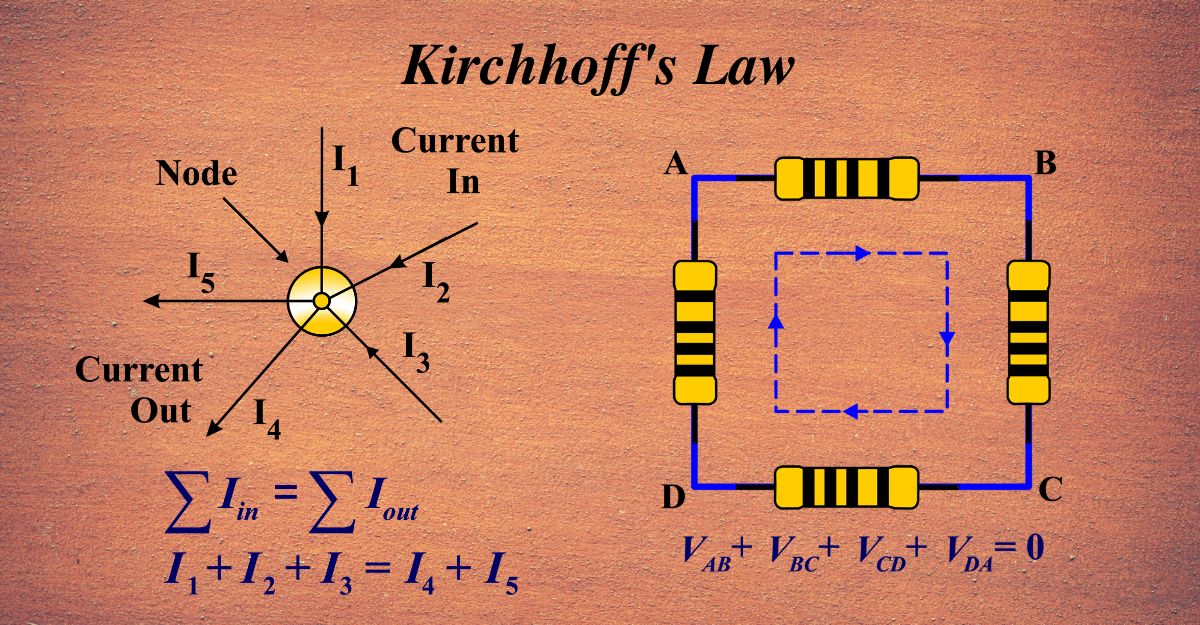
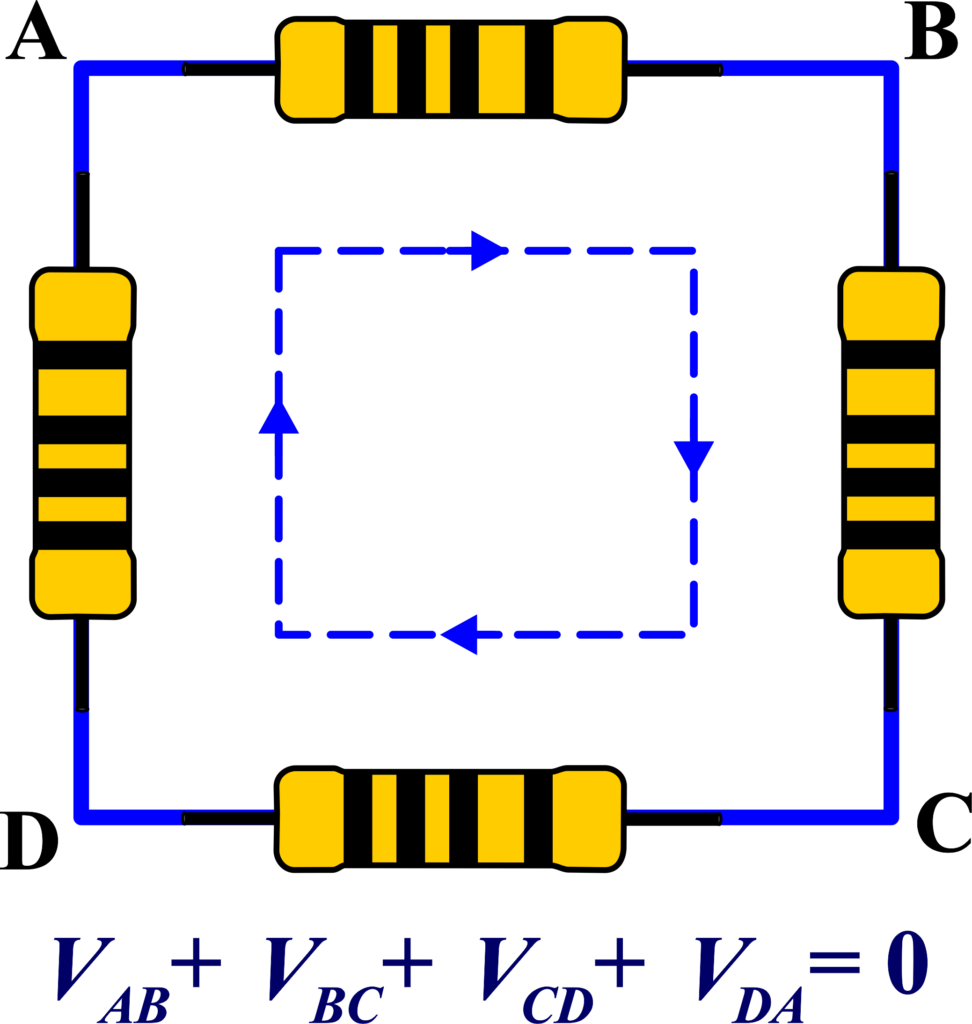
Kirchhoff’s first law, which deals with current at a junction, ensures that the current going into the junction must equal the sum of the currents leaving the junction. His second law, concerning voltage in a closed loop, asserts that the sum of the voltage differences within the loop equals zero.

These laws were originally obtained from experimental results and can be viewed as extensions of the conservation of charge and energy. They are accurate for DC circuits and for AC circuits at frequencies where the wavelengths of electromagnetic radiation are very large compared to the circuits.

Kirchhoff’s work laid the groundwork for future physicists and engineers to understand and design complex electrical systems. His laws are still taught to students around the world as they provide the essential principles needed to solve circuit problems.

What Are Kirchhoff’s Laws?

Kirchhoff’s Laws are like the traffic rules for electricity in circuits. They tell us how current and voltage behave as they travel through different paths in a circuit. These laws are based on two principles: conservation of charge and conservation of energy.

Kirchhoff’s Current Law (KCL):

Imagine a busy intersection in a city. Cars (current) enter and leave the intersection, but the total number of cars entering always equals the number leaving. This is what Kirchhoff’s Current Law, or the Junction Rule, says about electricity:

• At any junction point in a circuit, the sum of currents entering the junction must equal the sum of currents leaving.
• It’s like saying, “What goes in must come out,” ensuring that no electricity is lost at the junction.

Kirchhoff’s Voltage Law (KVL):

Now, think of a roller coaster loop. The cart (electric charge) goes up and down hills (components like resistors and batteries), but it ends up back where it started. Kirchhoff’s Voltage Law, or the Loop Rule, tells us that:

• The total voltage around any closed loop of a circuit must add up to zero.
• This means if you add up all the ‘ups’ and ‘downs’ the cart goes through, it balances out to a flat track.

Different Names of Kirchhoff’s Laws: These laws are known by a few names, which can be a bit confusing. Here’s a quick guide:

• Kirchhoff’s Current Law (KCL) is also called Kirchhoff’s First Law or the Junction Rule.
• Kirchhoff’s Voltage Law (KVL) is also known as Kirchhoff’s Second Law or the Loop Rule.

These laws are super useful because they help us figure out how much current is flowing through each part of a circuit and the voltage across each component. It’s like having a map and traffic rules for electricity, which makes analyzing complex circuits much easier.

Kirchhoff’s Current Law (KCL) or Kirchhoff’s First Law

“KCL states that the total current entering a junction (or node) in a circuit is exactly equal to the total current leaving the junction.“

Think of a junction as a room where electrical paths meet. Just like your friends at the party, electricity (current) flows into and out of this room. KCL ensures that all the current that comes in must go out, so none is lost or magically created.

This means if you add up all the currents going into the junction and compare it to the sum of currents leaving, they will be equal. By understanding KCL, you can better analyze circuits and predict how current will flow, which is crucial for any work involving electronics.

KCL is all about what happens at a junction, or a node, in an electrical circuit. A node is a point where three or more conductors meet. To derive the expression for KCL, we’ll use the principle of conservation of charge, which tells us that charge cannot be created or destroyed in an isolated system.

Consider a junction in a circuit where multiple currents converge. Let’s say I1, I2, I3, …, In are the currents flowing into the junction, and I1', I2', I3', …, Im' are the currents flowing out.

According to the conservation of charge, the total charge entering the junction must equal the total charge leaving it over any period of time. This means the sum of currents entering the node must be equal to the sum of currents leaving the node. We can express this as an equation:

\(\displaystyle \sum_{\text{entering}} I = \sum_{\text{leaving}} I’ \)

If we consider the direction of current entering the node as positive and leaving as negative (or vice versa), we can write the KCL equation as:

\(\displaystyle \sum I_{\text{entering}} – \sum I_{\text{leaving}} = 0 \)

This simplifies to the standard form of KCL, which is:

\(\displaystyle \sum I = 0 \)

Here, the summation (∑) symbol means to add up all the currents entering and leaving the node.

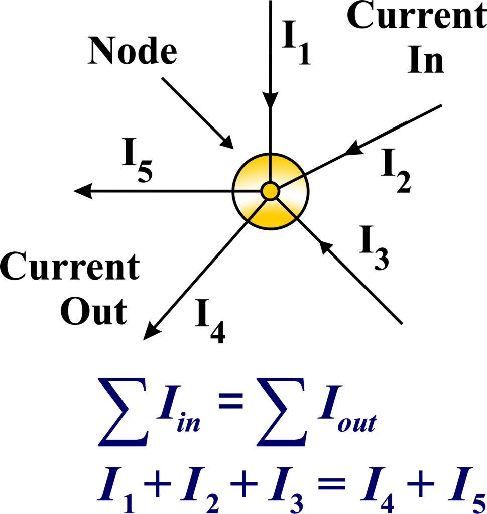
Example: A junction in an electrical circuit where three wires meet. We’ll label the currents flowing into the junction as I1, I2, and I3, and the currents flowing out as I4 and I5. Here’s what we know about the currents:

• I1 is 2A (amperes) flowing into the junction.
• I2 is 3A flowing into the junction.
• I3 is 4A flowing into the junction.
• I4 is 5A flowing out of the junction.
• I5 is 4A flowing out of the junction.

According to KCL, the total current entering the junction must equal the total current leaving the junction. So, we can set up the equation:

\(\displaystyle I1 + I2 + I3 = I4 + I5 \)

Plugging in the values we have:

\(\displaystyle 2A + 3A + 4A = 5A + 4A \)

When we add up the currents on each side, we get:

9A = 9A

This confirms that KCL holds for this junction—the sum of the currents entering the junction (9A) is equal to the sum of the currents leaving the junction (9A).

This law is very useful in circuit analysis because it allows us to calculate unknown currents if we know the others. For instance, if we didn’t know I3, but we knew all the other currents, we could rearrange the equation to solve for I3:

\(\displaystyle I3 = I4 + I5 – I1 – I2 \)

By understanding examples like this, you can apply KCL to solve for unknowns and analyze complex circuits in their studies and future work in electronics and electrical engineering.

Kirchhoff’s Voltage Law (KVL) or Kirchhoff’s Second Law

“KVL states that the sum of all the voltages around any closed loop in a circuit must equal zero.“

This means if you add up all the ‘ups’ (voltage gains) and ‘downs’ (voltage drops) in a loop, they should cancel each other out. KVL is like a financial budget for a road trip. Imagine you’re planning a trip with a certain amount of money, and you need to manage expenses so that by the end of the trip, you’re not overspending. Similarly, KVL helps us manage the ‘budget’ of voltages in a closed circuit.

Here, (V) represents the voltage, and the summation (∑) indicates that we add up all the voltages around the loop.

Example: Imagine you have a simple electrical circuit that forms a loop and consists of a battery and two resistors. The battery provides a voltage of (V_b), and the resistors have resistances (R₁) and (R₂). Let’s say the current flowing through the circuit is (I).

According to KVL, the sum of all voltages around the loop must be zero. So as we move around the loop, we’ll encounter the following changes in voltage:

When we move through the battery from negative to positive, we gain voltage (like climbing up a hill). This is a voltage gain of (V_b).

Moving through the resistor in the direction of the current, we experience a voltage drop (like going down a hill). This drop is (I × R₁) due to Ohm’s Law.

Similarly, moving through the second resistor, we have another voltage drop of (I × R₂).

Now, applying KVL, we write the equation for the loop:

\(\displaystyle V_b – I \times R_1 – I \times R_2 = 0 \)

This equation tells us that the voltage provided by the battery is used up by the resistors in the circuit. If we know the values of (V_b), (R₁), and (R₂), we can solve for the current (I) using this equation.

For example, if (V_b = 12V ), (R₁ = 2Ω), and (R₂ = 3Ω), the equation becomes:

\(\displaystyle 12V – I \times 2\Omega – I \times 3\Omega = 0 \)

Solving for (I), we get:

\(\displaystyle I = \frac{12V}{2\Omega + 3\Omega} = \frac{12V}{5\Omega} = 2.4A \)

So, the current flowing through the circuit is (2.4A). This example illustrates how KVL helps us understand the distribution of voltage in a circuit and calculate unknown quantities. It’s a practical application of the conservation of energy principle in electrical circuits.

Sign Conventions for Kirchhoff’s Law

Kirchhoff’s Current Law (KCL): When using KCL, we consider the current entering a junction as positive. Conversely, the current leaving a junction is considered negative. This helps us keep track of the flow of current and ensures that the algebraic sum of currents at a junction is zero.

Kirchhoff’s Voltage Law (KVL): When we traverse a loop and move from the negative to the positive terminal of a battery or any EMF source, we consider it as a voltage gain, and it’s assigned a positive sign.

If we move from the positive to the negative terminal, it’s a voltage drop, and we assign a negative sign. When moving in the direction of the current through a resistor, the potential drop (voltage drop) is negative, and it’s represented as (-IR).

When applying these rules, you’ll set up equations based on the paths you take around a circuit. It’s important to be consistent with your sign convention throughout your analysis. If you start by considering the current entry as positive, you must continue with that convention for the entire problem.

These conventions are like the grammar rules of circuit analysis—once you know them well, you can write the ‘sentences’ that describe any circuit’s behavior. And just like in language, consistency is key to making sure your ‘sentences’ (or equations) make sense!

Applications of Kirchhoff’s Laws

Kirchhoff’s Laws are incredibly useful in the world of physics and electrical engineering. Here’s how they apply to real-world scenarios :

Circuit Analysis: Kirchhoff’s Laws are the go-to tools for analyzing circuits that are too complex for simple series and parallel rules. They help in calculating unknown currents and voltages in various parts of a circuit. When a circuit isn’t working as expected, these laws can help identify where things are going wrong by checking the current and voltage at different points.

Design and Engineering: Engineers use Kirchhoff’s Laws to design electrical systems for buildings, vehicles, and electronics to ensure they are safe and efficient. By understanding the flow of current and distribution of voltage, engineers can optimize circuits for better performance.

Educational Tools: For students, Kirchhoff’s Laws are fundamental in learning about electricity and circuits. They form a basis for more advanced studies in physics and engineering. In physics labs, students use these laws to set up experiments and verify the behavior of circuits in practice.

Everyday Technology: The principles of Kirchhoff’s Laws are at play in the electronic circuits within all the gadgets and devices we use every day, from smartphones to kitchen appliances⁶.

Measurement Instruments: These laws are used to measure voltage and current in voltmeters and ammeters, essential tools for any electrical work.

Limitations of Kirchhoff’s Laws

Kirchhoff’s Laws are incredibly powerful for analyzing electrical circuits, but they do have some limitations.

Ideal Conditions Assumption: Kirchhoff’s Laws assume that the circuits are ideal, which means that the wires are perfect conductors with no resistance, so there’s no energy loss as current flows through them. The signals or changes in the circuit happen instantly without any delay.

High-Frequency Limitations: Kirchhoff’s Laws may not be accurate for high-frequency AC circuits. At high frequencies, the inductance and capacitance of the wires can’t be ignored, and the laws become less precise.

Time-Varying Fields: The laws are based on the assumption that the magnetic fields are constant over time. If there are time-varying magnetic fields, the laws need to be modified to take into account the induced EMF (electromotive force) that can arise.

In real circuits, there are factors like wire resistance, inductance, and capacitance that can affect the current and voltage. These factors can introduce discrepancies that Kirchhoff’s Laws don’t account for. While Kirchhoff’s Laws are great for analyzing simple to moderately complex circuits, they can become cumbersome and less practical for very complex circuits with many components and loops.

Also Read: Combination of Cells in Series and Parallel

Solved Examples

Problem 1: In a circuit, a loop contains three resistors (R₁ = 2 Ω), (R₂ = 4 Ω), and (R₃ = 6 Ω), and a battery of (V = 12 V). Calculate the current flowing through the loop.

Solution:

According to Kirchhoff’s Voltage Law (KVL), the sum of the potential differences (voltage) around any closed loop is zero. Therefore,

\(\displaystyle V – I R_1 – I R_2 – I R_3 = 0 \)
\(\displaystyle 12 – I(2 + 4 + 6) = 0 \)
\(\displaystyle 12 – I \cdot 12 = 0 \)
\(\displaystyle I = \frac{12}{12} = 1 \, \text{A} \)

The current flowing through the loop is (1 A).

Problem 2: At a junction in a circuit, three currents are meeting: (I₁ = 3 A) entering, (I₂ = 2 A) leaving, and (I₃) unknown and leaving the junction. Determine (I₃).

Solution: According to Kirchhoff’s Current Law (KCL), the sum of currents entering a junction is equal to the sum of currents leaving the junction.

\(\displaystyle I_1 = I_2 + I_3 \)
\(\displaystyle 3 \, \text{A} = 2 \, \text{A} + I_3 \)
\(\displaystyle I_3 = 3 \, \text{A} – 2 \, \text{A} \)
\(\displaystyle I_3 = 1 \, \text{A} \)

The current (I₃) is (1A).

Problem 3: In a circuit with two loops, the resistances are (R₁ = 3 Ω), (R₂ = 5 Ω), (R₃ = 2 Ω), and the voltages are (V₁ = 10 V), (V₂ = 5 V). Find the currents (I₁) and (I₂) in the loops.

Solution: Loop 1: (V₁) in series with (R₁) and (R₂)

\(\displaystyle 10 – 3I_1 – 5I_2 = 0 \quad \text{(1)} \)

Loop 2: (V₂) in series with (R₂) and (R₃)

\(\displaystyle 5 – 5I_1 – 2I_2 = 0 \quad \text{(2)} \)

From (2):

\(\displaystyle 5 = 5I_1 + 2I_2 \)
\(\displaystyle 2I_2 = 5 – 5I_1 \)
\(\displaystyle I_2 = \frac{5 – 5I_1}{2} \quad \text{(3)} \)

Substitute (3) into (1):

\(\displaystyle 10 – 3I_1 – 5\left(\frac{5 – 5I_1}{2}\right) = 0 \)
\(\displaystyle 10 – 3I_1 – \frac{25 – 25I_1}{2} = 0 \)
\(\displaystyle 10 – 3I_1 – 12.5 + 12.5I_1 = 0 \)
\(\displaystyle -2.5 + 9.5I_1 = 0 \)
\(\displaystyle 9.5I_1 = 2.5 \)
\(\displaystyle I_1 = \frac{2.5}{9.5} \approx 0.263 \, \text{A} \)

Using (I₁) in (3):

\(\displaystyle I_2 = \frac{5 – 5 \times 0.263}{2} \)
\(\displaystyle I_2 = \frac{5 – 1.315}{2} \)
\(\displaystyle I_2 \approx 1.8425 \, \text{A} \)

The currents are (\(\displaystyle I_1 \approx 0.263 \, \text{A} \)) and (\(\displaystyle I_2 \approx 1.8425 \, \text{A} \)).

Problem 4: In the circuit below, find the current flowing through each resistor using Kirchhoff’s Laws:

• (V₁ = 15 V), (V₂ = 10 V)
• (R₁ = 4 Ω), (R₂ = 6 Ω), (R₃ = 5 Ω)

Solution: Loop 1:

\(\displaystyle V_1 – I_1 R_1 – I_2 R_2 = 0 \)
\(\displaystyle 15 – 4I_1 – 6I_2 = 0 \quad \text{(1)} \)

Loop 2:

\(\displaystyle V_2 – I_2 R_2 – I_3 R_3 = 0 \)
\(\displaystyle 10 – 6I_2 – 5I_3 = 0 \quad \text{(2)} \)

Junction rule (assuming (I₁) splits into (I₂) and (I₃)):

\(\displaystyle I_1 = I_2 + I_3 \quad \text{(3)} \)

Substitute (I₃ = I₁ – I₂) from (3) into (2):

\(\displaystyle 10 – 6I_2 – 5(I_1 – I_2) = 0 \)
\(\displaystyle 10 – 6I_2 – 5I_1 + 5I_2 = 0 \)
\(\displaystyle 10 – I_2 – 5I_1 = 0 \)
\(\displaystyle I_2 = 10 – 5I_1 \)

Substitute (I₂ = 10 – 5I₁) into (1):

\(\displaystyle 15 – 4I_1 – 6(10 – 5I_1) = 0 \)
\(\displaystyle 15 – 4I_1 – 60 + 30I_1 = 0 \)
\(\displaystyle 26I_1 = 45 \)
\(\displaystyle I_1 = \frac{45}{26} \approx 1.731 \, \text{A} \)

Using (I₁):

\(\displaystyle I_2 = 10 – 5 \times 1.731 \)
\(\displaystyle I_2 \approx 1.345 \, \text{A} \)

Using (I₁) and (I₂) in (3):

\(\displaystyle I_3 = I_1 – I_2 \)
\(\displaystyle I_3 \approx 1.731 – 1.345 \)
\(\displaystyle I_3 \approx 0.386 \, \text{A} \)

The currents are (\(\displaystyle I_1 \approx 1.731 \, \text{A} \)), (\(\displaystyle I_2 \approx 1.345 \, \text{A} \)), and (\(\displaystyle I_3 \approx 0.386 \, \text{A} \)).

Problem 5: Determine the current through the galvanometer in a Wheatstone bridge circuit where (R₁ = 2 Ω), (R₂ = 3 Ω), (R₃ = 4 Ω), ( R4 = 6 Ω), and the battery voltage is (12 V).

Solution: In a balanced Wheatstone bridge:

\(\displaystyle \frac{R_1}{R_2} = \frac{R_3}{R_4} \)

\(\displaystyle \frac{2}{3} \neq \frac{4}{6} \)

Since the bridge is not balanced, there will be a current through the galvanometer. Let’s apply Kirchhoff’s Laws. Let (I) be the total current from the battery.

Applying KVL to the left loop:

\(\displaystyle 12 – 2I_1 – 3I_G = 0 \quad \text{(1)} \)

Applying KVL to the right loop:

\(\displaystyle 12 – 6I_2 – 4I_G = 0 \quad \text{(2)} \)

Using KCL at the junctions:

\(\displaystyle I = I_1 + I_2 \quad \text{(3)} \)
\(\displaystyle I_G = I_1 – I_2 \quad \text{(4)} \)

From (1):

\(\displaystyle 2I_1 + 3I_G = 12 \)
\(\displaystyle I_1 = \frac{12 – 3I_G}{2} \quad \text{(5)} \)

From (2):

\(\displaystyle 6I_2 + 4I_G = 12 \)
\(\displaystyle I_2 = \frac{12 – 4I_G}{6} \quad \text{(6)} \)

Substitute (5) and (6) into (4):

\(\displaystyle I_G = \frac{12 – 3I_G}{2} – \frac{12 – 4I_G}{6} \)
\(\displaystyle I_G = \frac{6 – 1.5I_G}{1} – \frac{2 – 0.667I_G}{1} \)
\(\displaystyle I_G = 3 – 1.5I_G + 0.667I_G \)
\(\displaystyle 2.5I_G = 3 \)
\(\displaystyle I_G \approx 1.2 \, \text{A} \)

The current through the galvanometer is approximately (1.2 A).

Problem 6: In a circuit, there are three resistors (R₁ = 2 Ω), (R₂ = 4 Ω), (R₃ = 8 Ω), and two batteries (V₁ = 10 V) and (V₂ = 5 V). Calculate the current through each resistor.

Solution: Loop 1: (V₁) in series with (R₁) and (R₂)

\(\displaystyle 10 – 2I_1 – 4I_2 = 0 \quad \text{(1)} \)

Loop 2: (V₂) in series with (R₂) and (R₃)

\(\displaystyle 5 – 4I_2 – 8I_3 = 0 \quad \text{(2)} \)

Junction rule:

\(\displaystyle I_1 = I_2 + I_3 \quad \text{(3)} \)

From (2):

\(\displaystyle 5 = 4I_2 + 8I_3 \)
\(\displaystyle 4I_2 = 5 – 8I_3 \)
\(\displaystyle I_2 = \frac{5 – 8I_3}{4} \quad \text{(4)} \)

Substitute (4) into (1):

\(\displaystyle 10 – 2I_1 – 4\left(\frac{5 – 8I_3}{4}\right) = 0 \)
\(\displaystyle 10 – 2I_1 – 5 + 8I_3 = 0 \)
\(\displaystyle 2I_1 – 8I_3 = 5 \)
\(\displaystyle I_1 = 4I_3 + 2.5 \quad \text{(5)} \)

Using (5) in (3):

\(\displaystyle 4I_3 + 2.5 = I_2 + I_3 \)
\(\displaystyle 4I_3 + 2.5 = \frac{5 – 8I_3}{4} + I_3 \)
\(\displaystyle 4I_3 + 2.5 = \frac{5 – 8I_3 + 4I_3}{4} \)
\(\displaystyle 4I_3 + 2.5 = 5 – 8I_3 + I_3 \)
\(\displaystyle 8I_3 + 8I_3 + 5I_3 = 5 – 8I_3 \)
\(\displaystyle I_3 \approx 0.26 \, \text{A} \)

Using (I₃):

\(\displaystyle I_1 = 4 \times 0.26 + 2.5 \)
\(\displaystyle I_1 \approx 3.54 \, \text{A} \)

Using (I₃):

\(\displaystyle I_2 = \frac{5 – 8 \times 0.26}{4} \)
\(\displaystyle I_2 \approx 0.68 \, \text{A} \)

The currents through the resistors are (\(\displaystyle I_1 \approx 3.54 \, \text{A} \)), (\(\displaystyle I_2 \approx 0.68 \, \text{A} \)), and (\(\displaystyle I_3 \approx 0.26 \, \text{A}\) ).

FAQs