The story of the Biot-Savart Law begins in the early 19th century with two French physicists, Jean-Baptiste Biot, and Félix Savart. These scientists were intrigued by the relationship between electricity and magnetism, a topic that was not well understood at the time.
In 1820, during a series of experiments, Biot and Savart discovered that electric currents create magnetic fields. This was a groundbreaking revelation because it linked two seemingly separate forces of nature. They observed that a magnetic compass needle was deflected when placed near a wire carrying an electric current. This deflection was evidence of a magnetic field generated by the electric current.
Biot and Savart conducted meticulous experiments to measure the magnetic field at various points around the current-carrying wire. They found that the strength and direction of the magnetic field depended on the distance from the wire and the shape of the current path.
Their work led to the formulation of the Biot-Savart Law, which mathematically describes the magnetic field produced by an electric current. This law was one of the first quantitative links between electricity and magnetism and laid the foundation for the field of electromagnetism.
The Biot-Savart Law was also instrumental in the development of Ampère’s Circuital Law and played a role in James Clerk Maxwell’s formulation of his famous equations, which unified the theories of electricity and magnetism.
What is Biot-Savart Law?
The Biot-Savart Law describes the magnetic field created by a current-carrying conductor. It provides a method to calculate the magnetic field at a point in space due to an electric current. Imagine you’re holding a hose that sprays water. The water represents the electric current, and the direction you’re pointing the hose is the direction of the current. Now, if you place a pinwheel near the stream of water, the pinwheel will start to spin. This spinning is similar to the magnetic field that’s created around a wire when an electric current flows through it.
The Biot-Savart Law helps us understand this “pinwheel effect” of magnetic fields around currents. It tells us that any moving electric charge (current) creates a magnetic field around it, just like the water from the hose creates motion in the air around the pinwheel.
Think of the current as a line of ants marching along a path. As they march, they create a little wind around them. The Biot-Savart Law tells us how strong that wind is and in which direction it blows, depending on how far you are from the path and where you’re standing.
The law gives us a formula that looks a bit complex but is just a way to calculate the strength and direction of this magnetic “wind” created by the current.
The formula is given by:
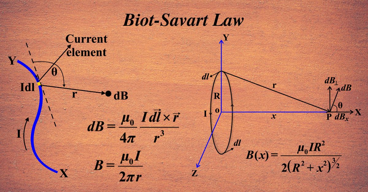
\(\displaystyle dB = \frac{\mu_0}{4\pi} \frac{Id\vec{l} \times \vec{r}}{r^3} \)
- (dB) is the infinitesimal magnetic field,
- (µ0) is the permeability of free space,
- (I) is the current,
- ( \(\displaystyle d\vec{l} \)) is the infinitesimal length of the conductor carrying the current,
- (\(\displaystyle\vec{r}\) ) is the position vector from the element to the point where the field is being calculated.
The cross product (×) in the formula is crucial. It tells us that the direction of the magnetic field (dB) is perpendicular to both the direction of the current (d𝐥) and the line from the wire to the point where we’re measuring (𝐫). To find this direction, you can use the right-hand rule: Point your thumb in the direction of the current, and your fingers in the direction of 𝐫. The direction your palm faces is the direction of the magnetic field.
Biot Savart law in Vector Form: In vector form, the law is expressed as:
\(\displaystyle \vec{B} = \frac{\mu_0}{4\pi} \int \frac{I d\vec{l} \times \vec{r}}{r^3} \)
This form allows us to calculate the magnetic field vector at any point in space due to a current-carrying wire. In physics, we often use arrows called vectors to represent things that have both a size and a direction, like the magnetic field. The Biot-Savart Law in vector form is like a detailed map that shows not just how strong the magnetic field is at different points, but also the exact direction it points in.
Biot Savart Law Derivation
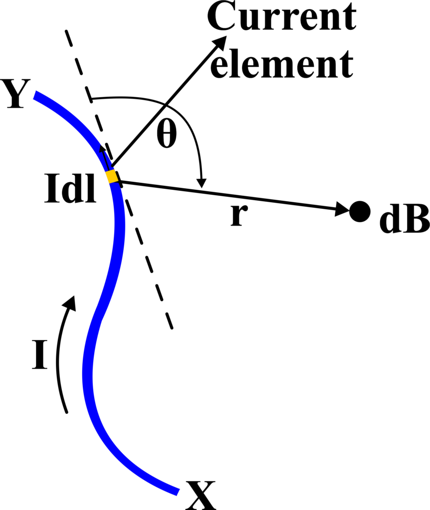
The derivation involves integrating the contributions of magnetic fields from all infinitesimal current elements along the conductor. Imagine you have a wire through which an electric current (I) is flowing. Now, we want to find out the magnetic field (\(\displaystyle \vec{B} \)) created by this current at a point in space.
We start by considering a very small segment of the wire, which we’ll call a current element, represented by (\(\displaystyle d\vec{l} \)). This tiny piece of the wire carries a small part of the current.
According to the Biot-Savart Law, this current element creates a tiny magnetic field (dB) at a point (P), located at a distance (r) from the element. The direction of (dB) is perpendicular to both (\(\displaystyle d\vec{l} \)) and the line from the current element to point (P).
The magnitude of this tiny magnetic field is given by the formula:
\(\displaystyle dB = \frac{\mu_0}{4\pi} \frac{I \, d\vec{l} \times \vec{r}}{r^3} \)
where (\(\displaystyle\mu_0 \)) is the permeability of free space, and (\(\displaystyle \vec{r}\) ) is the position vector from the current element to point (P).
Since we’re only looking at a tiny segment, we need to add up the magnetic fields from all such segments along the wire. This is done by integrating the expression for (dB) over the length of the wire.
After integrating, we get the full expression for the magnetic field (\(\displaystyle\vec{B}\) ) at point (P):
\(\displaystyle \vec{B} = \frac{\mu_0}{4\pi} \int \frac{I \, d\vec{l} \times \vec{r}}{r^3} \)
This integral sums up the contributions from all parts of the wire to give us the total magnetic field at point (P). In real-life problems, we often deal with wires of specific shapes (like straight lines or loops), so we can simplify this integral for those cases to make the calculation easier.
Relationship between Biot-Savart law and Coulomb’s law
Both laws describe the force fields generated by sources (magnetic fields by currents and electric fields by charges) and both decrease with the square of the distance from the source.
Coulomb’s Law deals with electrostatic forces between stationary charges. It tells us that the electric force between two charges is directly proportional to the product of the charges and inversely proportional to the square of the distance between them.
The Biot-Savart Law applies to magnetic fields created by moving charges (currents). It helps us calculate the magnetic field at a point in space due to a current-carrying conductor.
Similarities: Here are some similarities between the two laws:
- Inverse Square Relationship: Both laws show that the force or field strength decreases with the square of the distance from the source. In Coulomb’s Law, the electric force diminishes as the distance between charges increases, and in the Biot-Savart Law, the magnetic field weakens as you move away from the current-carrying wire.
- Superposition Principle: Both laws follow the principle of superposition, which means that if there are multiple sources (charges for Coulomb’s Law and current elements for the Biot-Savart Law), you can add up the effects from each source to find the total field at any point.
Differences:
- Static vs. Moving Charges: Coulomb’s Law is concerned with static (stationary) charges, while the Biot-Savart Law is used when charges are in motion, i.e., when there is a current.
- Electric vs. Magnetic Fields: Coulomb’s Law calculates the electric field and force between charges, whereas the Biot-Savart Law calculates the magnetic field due to currents.
Fundamental Constants: There’s also a relationship between the constants involved in both laws: Coulomb’s Law describes the electric force between two stationary charges. The formula is:
\(\displaystyle F = k \frac{q_1 q_2}{r^2} \)
- (F) is the electric force,
- (k) is Coulomb’s constant (\(\displaystyle k = \frac{1}{4\pi\varepsilon_0} \)),
- (q1) and (q2) are the charges,
- (r) is the distance between the charges,
- (\(\displaystyle \varepsilon_0 \)) is the permittivity of free space.
The Biot-Savart Law gives us the magnetic field due to a current element. The formula is:
\(\displaystyle dB = \frac{\mu_0}{4\pi} \frac{Id\vec{l} \times \vec{r}}{r^3} \)
The constants (µ0) and (\(\displaystyle\varepsilon_0\)) are related to each other and to the speed of light (c) in a vacuum by the equation:
\(\displaystyle c = \frac{1}{\sqrt{\mu_0\varepsilon_0}} \)
This shows a deep connection between electric and magnetic phenomena. The speed of light being related to these constants is a fundamental aspect of electromagnetism.
To derive the relationship between the constants in both laws, we can start with the expression for the speed of light:
\(\displaystyle c^2 = \frac{1}{\mu_0\varepsilon_0} \)
Rearranging this, we get:
\(\displaystyle \mu_0\varepsilon_0 = \frac{1}{c^2} \)
Now, if we look at Coulomb’s constant (k), we can express it using (\(\displaystyle\varepsilon_0 \)):
\(\displaystyle k = \frac{1}{4\pi\varepsilon_0} \)
Substituting (\(\displaystyle\varepsilon_0 \)) from the speed of light equation, we get:
\(\displaystyle k = \frac{c^2}{4\pi\mu_0} \)
This shows that Coulomb’s constant (k) and the constant (µ0) from the Biot-Savart Law are inversely related to the speed of light.
By understanding the relationship between (µ0) and (\(\displaystyle\varepsilon_0 \)), students can see how the electric and magnetic fields are part of the same fundamental force, electromagnetism, and how changes in one can affect the other.
The Biot–Savart Law, Ampère’s Circuital Law, and Gauss’s Law for Magnetism
The Biot-Savart Law is consistent with Ampère’s Circuital Law and Gauss’s Law for Magnetism, which are fundamental to magnetostatics.
1) Biot–Savart Law and Ampère’s Circuital Law: Both laws describe the magnetic field due to currents. The Biot–Savart Law is used for calculating the magnetic field at a point, while Ampère’s Circuital Law is used when there’s symmetry, and you want to know the field along a path. Ampère’s Law can be derived from the Biot–Savart Law in situations with high symmetry.
The Biot–Savart Law gives us the magnetic field (\(\displaystyle\vec{B}\)) at a point in space due to a small current element (\(\displaystyle Id\vec{l} \)):
\(\displaystyle dB = \frac{\mu_0}{4\pi} \frac{Id\vec{l} \times \vec{r}}{r^3} \)
Ampère’s Circuital Law states that the line integral of the magnetic field (\(\displaystyle\vec{B}\)) around any closed loop is equal to the permeability of free space (µ0) times the electric current (I) passing through the loop:
\(\displaystyle \oint \vec{B} \cdot d\vec{l} = \mu_0 I \)
Consider a long, straight wire carrying a current (I). We want to find the magnetic field at a point a distance (r) away from the wire. Calculate the magnetic field at the point using the Biot–Savart Law. For a straight wire, the law simplifies to:
\(\displaystyle dB = \frac{\mu_0}{4\pi} \frac{I dl \sin(\theta)}{r^2} \)
where (θ) is the angle between (\(\displaystyle d\vec{l} \)) and (\(\displaystyle \vec{r} \)), which is 90 degrees for all elements of a straight wire.
To find the total magnetic field (B), integrate (dB) over the length of the wire. For an infinitely long wire, this gives us:
\(\displaystyle B = \frac{\mu_0 I}{2\pi r} \)
Now, apply Ampère’s Circuital Law by taking a circular path around the wire with radius (r). The line integral of (B) around this path is:
\(\displaystyle \oint \vec{B} \cdot d\vec{l} = B(2\pi r) = \mu_0 I \)
Notice that the expression for (B) from the Biot–Savart Law matches the result from Ampère’s Circuital Law for this symmetrical case. The Biot–Savart Law can be used to derive Ampère’s Circuital Law for cases with high symmetry, such as an infinitely long straight wire. In more complex scenarios without symmetry, the Biot–Savart Law is used to calculate the magnetic field at a point, while Ampère’s Circuital Law provides a quick way to calculate the field along a path when symmetry is present.
2) Ampère’s Circuital Law and Gauss’s Law for Magnetism: Ampère’s Law is consistent with Gauss’s Law for Magnetism because it inherently considers the closed nature of magnetic field lines. When you use Ampère’s Law to calculate the magnetic field along a closed loop, you’re acknowledging that the magnetic field lines form closed loops, as stated by Gauss’s Law.
3) Biot–Savart Law and Gauss’s Law for Magnetism: The Biot–Savart Law, while used for point calculations, also respects the principle that magnetic field lines are closed loops, which is the essence of Gauss’s Law for Magnetism.
The Biot–Savart Law allows us to calculate the magnetic field generated by a current-carrying wire. It states that the magnetic field (\(\displaystyle\vec{B}\)) at a point in space is proportional to the current (I), the length of the wire element (\(\displaystyle d\vec{l} \)), and inversely proportional to the square of the distance from the wire element to the point where the field is measured.
Gauss’s Law for Magnetism states that the net magnetic flux through any closed surface is zero. This implies that magnetic field lines do not begin or end at any point (i.e., there are no magnetic monopoles) and that they form closed loops.
- Magnetic Field Lines: According to the Biot–Savart Law, the magnetic field lines created by a current-carrying wire are circular and centered on the wire. If we were to draw a closed surface around the wire, such as a cylinder, the magnetic field lines would enter one end of the surface and exit the other, never starting or stopping within the surface.
- Applying Gauss’s Law: When we apply Gauss’s Law for Magnetism to this closed surface, we find that the net magnetic flux through the surface is zero because the number of field lines entering the surface is equal to the number leaving it.
- Consistency Between Laws: This consistency shows the relationship between the Biot–Savart Law and Gauss’s Law for Magnetism. The Biot–Savart Law describes how the magnetic field is generated and its configuration in space, while Gauss’s Law for Magnetism confirms the fundamental nature of magnetic field lines as closed loops.
The Biot–Savart Law provides the detailed behavior of magnetic fields around currents, and Gauss’s Law for Magnetism provides a global statement about the nature of magnetic fields. Both laws are in agreement and together give a complete description of the magnetic field in and around current-carrying conductors.
Together, these laws give us a complete picture of how magnetic fields behave around electric currents and help us understand the fundamental nature of magnetism.
Applications of Biot – Savart Law
The magnetic field on the axis of a circular loop
Let’s discuss the application of the Biot–Savart Law to find the magnetic field on the axis of a circular loop. Imagine you have a circular loop of wire through which a current ( I ) is flowing. We want to find out what the magnetic field is like right at the center of this loop and along its axis.
At the Center of the Loop:
Imagine a circular loop of wire with radius (R) lying flat on a table. A current (I) flows through this loop. We want to find the magnetic field (B) at the very center of this loop. The Biot–Savart Law tells us that a small segment of current (\(\displaystyle Id\vec{l} \)) creates a small magnetic field (dB) at a point in space.
The law is given by:
\(\displaystyle dB = \frac{\mu_0}{4\pi} \frac{Id\vec{l} \times \vec{r}}{r^3} \)
where (µ0) is the permeability of free space, (\(\displaystyle d\vec{l}\) ) is the length of the current element, and (\(\displaystyle \vec{r}\) ) is the position vector from the current element to the point where we’re calculating the field.
At the center of the loop, the symmetry of the setup simplifies our calculations. The magnetic field contributions (dB) from each segment of the loop will have the same magnitude because each segment is equidistant from the center. Additionally, the direction of each (dB) will be perpendicular to the plane of the loop due to the right-hand rule.
To find the total magnetic field (B) at the center, we sum up the contributions from all the current elements around the loop. Due to the symmetry, the horizontal components of (dB) cancel out, and only the vertical components add up.
Since the angle (θ) between (\(\displaystyle d\vec{l} \)) and (\(\displaystyle \vec{r} \)) is 90 degrees, (sin(θ) = 1), and the distance (r) is the radius (R) of the loop, the expression for (dB) simplifies to:
\(\displaystyle dB = \frac{\mu_0}{4\pi} \frac{I dl}{R^2} \)
Integrating this around the entire loop gives us the total magnetic field (B) at the center:
\(\displaystyle B = \int dB = \frac{\mu_0}{4\pi} \frac{I}{R^2} \int dl \)
Since the integral of (dl) around the loop is the circumference (\(\displaystyle 2\pi R \)), we get:
\(\displaystyle B = \frac{\mu_0}{4\pi} \frac{I}{R^2} (2\pi R) \)
Simplifying this, we find that the (R) in the denominator cancels out one (R) from the circumference, leaving us with:
\(\displaystyle B = \frac{\mu_0 I}{2R} \)
This is the magnetic field at the center of the circular loop. This formula shows that the magnetic field at the center of a circular loop is directly proportional to the current and inversely proportional to the radius of the loop.
Along the Axis:
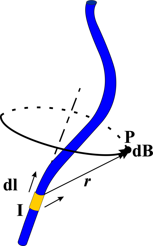
Imagine a circular loop of wire with radius (R) lying flat on a table. A current (I) flows through this loop. We want to find the magnetic field (B) at a point (P) along the axis of the loop, a distance (x) from the center of the loop.
The Biot–Savart Law tells us how to find the magnetic field (dB) created by a small segment of current-carrying wire:
\(\displaystyle dB = \frac{\mu_0}{4\pi} \frac{Id\vec{l} \times \vec{r}}{r^3} \)
Due to symmetry, the radial components of (dB) cancel out, and only the axial components contribute to the net field at point (P). The axial component of (dB) is
\(\displaystyle dB_{\text{axial}} = dB \cos(\theta) \)
where (θ) is the angle between (\(\displaystyle d\vec{l} \)) and (\(\displaystyle \vec{r} \)).
The axial component is given by:
$$ dB_{\text{axial}} = dB \cos(\theta) = \frac{\mu_0}{4\pi} \frac{I dl \sin(\phi) \cos(\theta)}{(R^2 + x^2)} $$
Here, (\(\displaystyle \phi \)) is the angle between (\(\displaystyle d\vec{l}\) ) and the plane of the loop (which is ( 90∘)), making (\(\displaystyle \sin(\phi) = 1 \)). The angle (θ) can be related to (R) and (x) by the right triangle formed by (R), (x), and (r), giving us
\(\displaystyle \cos(\theta) = \frac{x}{\sqrt{R^2 + x^2}} \).
We integrate (dBaxial) over the entire loop to find the total magnetic field (B) at point (P):
\(\displaystyle B(x) = \int dB_{\text{axial}} = \frac{\mu_0 I x}{4\pi (R^2 + x^2)} \int_0^{2\pi} dl \)
Since the integral of (dl) around the loop is the circumference (\(\displaystyle 2\pi R \)), we get:
\(\displaystyle B(x) = \frac{\mu_0 I x}{4\pi (R^2 + x^2)} (2\pi R) \)
Simplifying this expression, we find:
\(\displaystyle B(x) = \frac{\mu_0 I R^2}{2(R^2 + x^2)^{3/2}} \)
This is the magnetic field at a distance (x) from the center along the axis of the circular loop. This formula shows that the magnetic field along the axis of a circular loop decreases as you move away from the center and depends on the radius of the loop and the current flowing through it.
Magnetic field due to a finite straight wire
Imagine a straight wire of length (L) lying horizontally. A current (I) flows through this wire. We want to find the magnetic field (B) at a point (P) that is at a perpendicular distance (r) from the midpoint of the wire.
The Biot–Savart Law gives us the differential magnetic field (dB) created by a small current element (\(\displaystyle Id\vec{l} \)):
\(\displaystyle dB = \frac{\mu_0}{4\pi} \frac{Id\vec{l} \times \vec{r}}{r^3} \)
Here, (µ0) is the permeability of free space, (\(\displaystyle d\vec{l} \)) is the infinitesimal length of the wire, and (\(\displaystyle \vec{r} \)) is the position vector from the wire to the point (P).
For a straight wire, (\(\displaystyle d\vec{l}\)) and (\(\displaystyle \vec{r} \)) are perpendicular, so (\(\displaystyle d\vec{l} \times \vec{r} \)) simplifies to (\(\displaystyle dl \cdot r \)). The magnitude of (dB) is then:
\(\displaystyle dB = \frac{\mu_0}{4\pi} \frac{I dl r}{r^3} = \frac{\mu_0}{4\pi} \frac{I dl}{r^2} \)
To find the total magnetic field (B), we integrate (dB) over the length of the wire. If we consider the wire to extend from (-L/2) to (L/2), the integration limits are from (-L/2) to (L/2).
The integration leads to the expression for the magnetic field (B) at point (P):
\(\displaystyle B = \int_{-L/2}^{L/2} \frac{\mu_0}{4\pi} \frac{I dl}{r^2} \)
After integrating, we get:
\(\displaystyle B = \frac{\mu_0 I}{4\pi r} \left[ \ln \left( \frac{L/2 + r}{L/2 – r} \right) \right] \)
This is the magnetic field at a distance (r) from a finite straight wire of length (L) carrying a current (I). This derivation shows how we use the Biot–Savart Law to calculate the magnetic field due to a finite straight wire.
Importance of Biot-Savart Law
Understanding Magnetic Fields: The Biot-Savart Law is crucial for understanding how magnetic fields are generated by moving charges, or currents. It provides a direct method to calculate the magnetic field at any point in space due to a current-carrying conductor. This is essential for many applications in physics and engineering.
Real-World Applications: The Biot-Savart Law has numerous practical applications. It’s used in designing electric motors, generators, and inductors. It also helps in understanding the behavior of devices ranging from simple compasses to complex MRI machines. Knowing this law helps students appreciate the real-world impact of physics.
Predictive Power: With the Biot-Savart Law, students can predict the magnetic field produced by any configuration of currents. This predictive power is not just academic; it’s used in designing circuits and electrical devices, ensuring they operate safely and efficiently.
This law lays the groundwork for more advanced concepts in physics. It’s one of the first steps toward understanding Maxwell’s equations, which unify electricity, magnetism, and light. A solid grasp of the Biot-Savart Law is vital for any student wishing to delve deeper into the study of electromagnetism or pursue a career in related fields.
Learning to apply the Biot-Savart Law enhances problem-solving skills. Students learn to break down complex problems into smaller parts, calculate the effects of each part, and then integrate these to find a solution. These skills are transferable to many other areas of study and work.
The Biot-Savart Law helps illustrate the interconnectedness of electric and magnetic forces. It shows students that these forces are not isolated phenomena but are closely related aspects of the electromagnetic force, one of the four fundamental forces in the universe.
Also Read: Ampère’s Law
Solved Examples
Problem 1: A circular loop of radius (R = 10 cm) carries a current (I = 5 A). Calculate the magnetic field at a point (20 cm) from the center of the loop along its axis.
Solution: The magnetic field (B) on the axis of a circular loop at a distance (x) from the center is given by:
\(\displaystyle B = \frac{\mu_0 I R^2}{2 (R^2 + x^2)^{3/2}} \)
Given: \(\displaystyle\mu_0 = 4\pi \times 10^{-7} \, \text{T} \cdot \text{m/A}\)
\(\displaystyle B = \frac{4\pi \times 10^{-7} \times 5 \times (0.1)^2}{2 [(0.1)^2 + (0.2)^2]^{3/2}} \)
\(\displaystyle B = \frac{4\pi \times 10^{-7} \times 5 \times 0.01}{2 (0.01 + 0.04)^{3/2}} \)
\(\displaystyle B = \frac{20\pi \times 10^{-7} \times 0.01}{2 (0.05)^{3/2}} \)
\(\displaystyle B = \frac{20\pi \times 10^{-9}}{2 \times 0.01118} \)
\(\displaystyle B = \frac{20\pi \times 10^{-9}}{0.02236} \)
\(\displaystyle B \approx \frac{62.83 \times 10^{-9}}{0.02236} \)
\(\displaystyle B \approx 2.81 \times 10^{-6} \, \text{T} \)
The magnetic field at a point (20 cm) from the center of the loop along its axis is (\(\displaystyle 2.81 \times 10^{-6} \, \text{T} \)).
Problem 2: A thin straight wire of length (L = 1 m) carries a uniform linear charge density (\(\displaystyle \lambda = 1 \, \mu \text{C/m} \)). Calculate the electric field at a point located at the perpendicular bisector of the wire at a distance (r = 0.5 m).
Solution: By Coulomb’s law, the electric field (E) at a distance (r) from a line of charge is given by:
\(\displaystyle E = \frac{\lambda}{2 \pi \epsilon_0 r} \)
\(\displaystyle E = \frac{1 \times 10^{-6}}{2 \pi \times 8.854 \times 10^{-12} \times 0.5} \)
\(\displaystyle E = \frac{10^{-6}}{2 \pi \times 4.427 \times 10^{-12}} \)
\(\displaystyle E = \frac{10^{-6}}{27.78 \times 10^{-12}} \)
\(\displaystyle E \approx 3.6 \times 10^4 \, \text{N/C} \)
The electric field at the point located at the perpendicular bisector of the wire is (\(\displaystyle 3.6 \times 10^4 \, \text{N/C}\) ).
Problem 3: A finite straight wire of length (L = 50 cm) carries a current (I = 10 A). Calculate the magnetic field at a point (P) located (10cm) perpendicular to the midpoint of the wire.
Solution: For a finite straight wire, the magnetic field (B) at a perpendicular distance (r) from the midpoint is given by:
\(\displaystyle B = \frac{\mu_0 I}{4 \pi r} \left( \sin \theta_1 + \sin \theta_2 \right) \)
For a wire segment of length (L), and a perpendicular distance (r) from the midpoint:
\(\displaystyle \theta_1 = \theta_2 = \arctan\left(\frac{L/2}{r}\right) \)
Given: (L = 0.5m), (r = 0.1 m), (I = 10A), \(\displaystyle \theta_1 = \theta_2 = \arctan\left(\frac{0.25}{0.1}\right) = \arctan(2.5) \approx 68.2^\circ \)
\(\displaystyle B = \frac{4\pi \times 10^{-7} \times 10}{4\pi \times 0.1} \left( \sin 68.2^\circ + \sin 68.2^\circ \right) \)
\(\displaystyle B = \frac{10 \times 10^{-7}}{0.1} \times 2 \times 0.93 \)
\(\displaystyle B = 2 \times 10^{-6} \times 0.93 \)
\(\displaystyle B \approx 1.86 \times 10^{-6} \, \text{T} \)
The magnetic field at the point (10 cm) perpendicular to the midpoint of the wire is (\(\displaystyle 1.86 \times 10^{-6} \, \text{T} \)).
Problem 4: Calculate the magnetic field at the center of a semi-circular arc of radius (10 cm) carrying a current of (15A).
Solution: For a semi-circular arc of radius (R) carrying a current (I), the magnetic field (B) at the center is given by:
\(\displaystyle B = \frac{\mu_0 I}{4R} \)
\(\displaystyle B = \frac{4\pi \times 10^{-7} \times 15}{4 \times 0.1} \)
\(\displaystyle B = \frac{4\pi \times 10^{-7} \times 15}{0.4} \)
\(\displaystyle B = \frac{60\pi \times 10^{-7}}{0.4} \)
\(\displaystyle B = \frac{60\pi \times 10^{-7}}{0.4} \)
\(\displaystyle B = 15\pi \times 10^{-6} \, \text{T} \)
\(\displaystyle B \approx 4.71 \times 10^{-5} \, \text{T} \)
The magnetic field at the center of the semi-circular arc is (\(\displaystyle 4.71 \times 10^{-5} \, \text{T}\) ).
Problem 5: A circular current loop of radius (20 cm) carries a current of (10 A). Calculate the magnetic field at a point on the axis of the loop at a distance equal to the radius of the loop.
Solution: The magnetic field (B) on the axis of a circular loop at a distance (x) from the center is given by:
\(\displaystyle B = \frac{\mu_0 I R^2}{2 (R^2 + x^2)^{3/2}} \)
Given: (R = 0.2 m), (I = 10 A), (x = 0.2 m), (\(\displaystyle\mu_0 = 4\pi \times 10^{-7} \, \text{T} \cdot \text{m/A}\))
\(\displaystyle B = \frac{4\pi \times 10^{-7} \times 10 \times (0.2)^2}{2 [(0.2)^2 + (0.2)^2]^{3/2}} \)
\(\displaystyle B = \frac{4\pi \times 10^{-7} \times 10 \times 0.04}{2 (0.08)^{3/2}} \)
\(\displaystyle B = \frac{4\pi \times 10^{-7} \times 10 \times 0.04}{2 \times 0.02263} \)
\(\displaystyle B = \frac{4\pi \times 10^{-7} \times 10 \times 0.04}{0.04526} \)
\(\displaystyle B = \frac{1.6\pi \times 10^{-6}}{0.04526} \)
\(\displaystyle B \approx 1.11 \times 10^{-5} \, \text{T} \)
The magnetic field at the point on the axis of the loop at a distance equal to the radius of the loop is (\(\displaystyle 1.11 \times 10^{-5} \, \text{T}\) ).
Problem 6: A straight wire segment of length (60 cm) carries a current of (5 A). Calculate the magnetic field at a point (30cm) perpendicular to one end of the wire.
Solution: For a finite straight wire, the magnetic field (B) at a perpendicular distance (r) from one end of the wire is given by:
\(\displaystyle B = \frac{\mu_0 I}{4 \pi r} (\sin \theta_1 + \sin \theta_2) \)
Given: (L = 0.6 m), (r = 0.3 m), (I = 5 A), (\(\displaystyle \mu_0 = 4\pi \times 10^{-7} \, \text{T} \cdot \text{m/A} \))
\(\displaystyle\theta_1 = 0 \)
\(\displaystyle \theta_2 = \arctan\left(\frac{L}{r}\right) = \arctan\left(\frac{0.6}{0.3}\right) = \arctan(2) \approx 63.43^\circ \)
\(\displaystyle B = \frac{4\pi \times 10^{-7} \times 5}{4\pi \times 0.3} (\sin 0^\circ + \sin 63.43^\circ) \)
\(\displaystyle B = \frac{5 \times 10^{-7}}{0.3} \times \sin 63.43^\circ \)
\(\displaystyle B = \frac{5 \times 10^{-7}}{0.3} \times 0.89 \)
\(\displaystyle B = 1.48 \times 10^{-6} \, \text{T} \)
The magnetic field at a point (30 cm) perpendicular to one end of the wire is (\(\displaystyle 1.48 \times 10^{-6} \, \text{T} \)).
FAQs
What is the Biot-Savart Law and what does it explain?
The Biot-Savart Law explains how to calculate the magnetic field produced by a small segment of a current-carrying conductor at a specific point in space. It describes how the magnetic field depends on the magnitude and direction of the current, the length of the conductor segment, and the distance from the segment to the point where the field is measured.
How does the Biot-Savart Law differ from Ampere’s Law?
The Biot-Savart Law provides a detailed method for calculating the magnetic field produced by any segment of current-carrying wire, making it suitable for complex geometries. Ampere’s Law, on the other hand, is more useful for symmetrical situations, where it can simplify the calculation of the magnetic field around conductors with high symmetry, such as solenoids and toroids.
Why is the Biot-Savart Law important in electromagnetism?
The Biot-Savart Law is crucial in electromagnetism because it gives a direct way to calculate the magnetic field generated by a current, which is fundamental in understanding and designing electrical devices such as motors, generators, and transformers. It also helps in analyzing the magnetic effects of current distributions in various practical applications.
How does the Biot-Savart Law apply to a current loop?
When applied to a current loop, the Biot-Savart Law helps determine the magnetic field at any point around the loop. For instance, it can be used to calculate the magnetic field along the axis of a circular loop, showing how the field varies with distance from the center of the loop.
How can the Biot-Savart Law be used to explain the magnetic field created by a straight current-carrying wire?
By applying the Biot-Savart Law to a straight current-carrying wire, one can derive the magnetic field at any point around the wire. This field forms concentric circles around the wire, with the direction given by the right-hand rule and the strength decreasing with distance from the wire.
What are the limitations of the Biot-Savart Law in practical applications?
The Biot-Savart Law can be complex to apply to large or intricate current distributions because it requires integrating over the entire current-carrying conductor. In such cases, simplifications or approximations, such as using Ampere’s Law for symmetrical situations, are often more practical. Additionally, it doesn’t account for the relativistic effects at high velocities.