
The early 19th century was an era of rapid progress in understanding electricity and magnetism. Before Faraday, scientists like Hans Christian Ørsted and André-Marie Ampère had already laid the groundwork by discovering that electric currents affect magnetic needles and that currents could attract or repel each other.
Michael Faraday, born in 1791, was not formally educated in the sciences. Yet, his natural curiosity and meticulous experimentation led him to become one of the most influential scientists in history. Working at the Royal Institution in London, Faraday was fascinated by the idea of converting magnetism into electricity.
In 1831, Faraday conducted a series of experiments that would change the course of science. He discovered that when he moved a magnet through a loop of wire, an electric current flowed in the wire. This was the first time anyone had generated electricity from magnetism, a phenomenon he called electromagnetic induction.
Faraday’s laws laid the foundation for electric generation and paved the way for inventions like the dynamo and the transformer. His work also inspired James Clerk Maxwell, who later used Faraday’s principles as a basis for his own set of equations—Maxwell’s equations—which fully describe the principles of electromagnetism.
Today, Faraday’s discoveries are fundamental to the technologies that power our world. From the electricity that lights our homes to the wireless signals that connect our phones, Faraday’s legacy lives on in the electromagnetic waves that surround us.
Faraday’s Laws of Electromagnetic Induction
Faraday’s first law
“ Whenever a conductor is placed in a varying magnetic field, an electromotive force (emf) is induced in the conductor. If the conductor circuit is closed, a current is induced, which is called the induced current.”
To understand this law, let us consider an example of a coil of wire connected to a galvanometer, which is a device that measures small currents. A bar magnet is moved towards and away from the coil, as shown in the figure below.
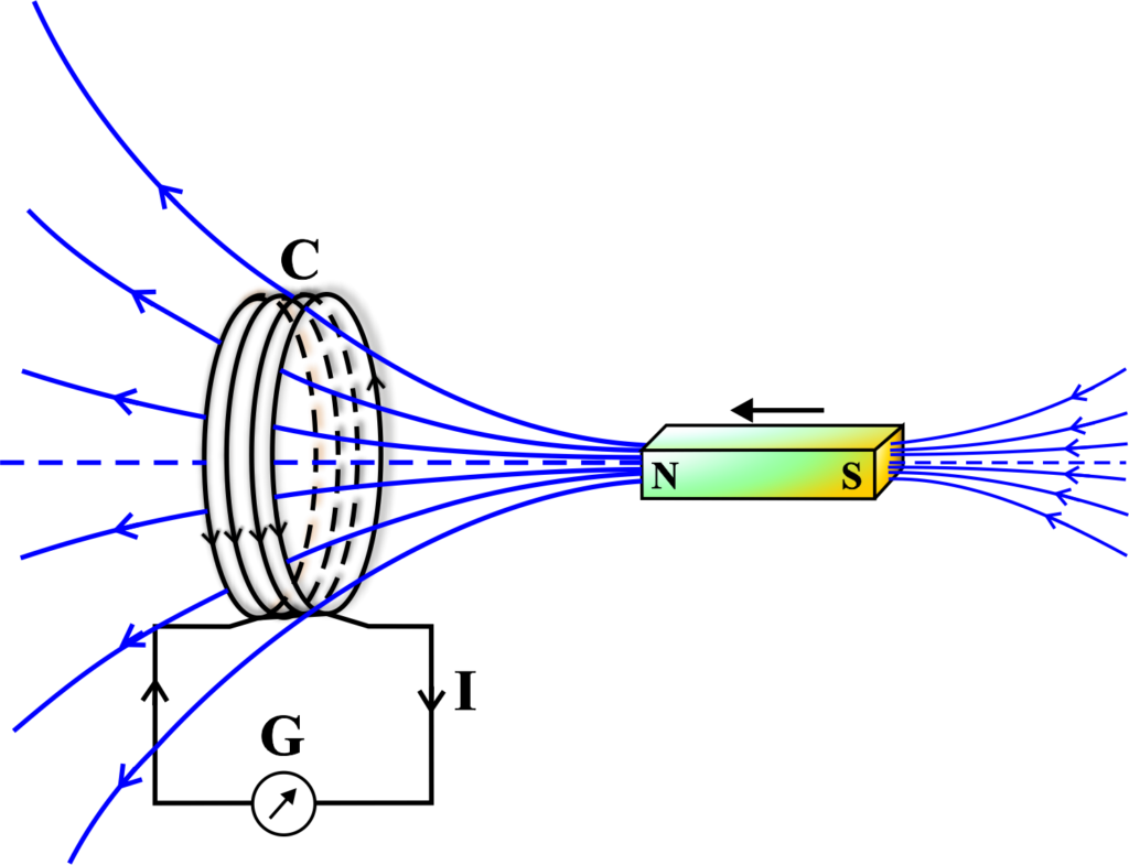
When the magnet is moved towards the coil, the magnetic flux through the coil increases. The magnetic flux is the product of the magnetic field and the area of the coil perpendicular to the field.
According to Faraday’s first law, this change in flux induces an emf in the coil, which causes a current to flow in the coil.
The direction of the current is such that it creates a magnetic field that opposes the increase in flux. This is according to Lenz’s law, which states that the induced current opposes the change that produces it. The galvanometer pointer shows a deflection, indicating the presence of current in the coil.
When the magnet is moved away from the coil, the magnetic flux through the coil decreases. This also induces an emf in the coil, which causes a current to flow in the opposite direction. The direction of the current is such that it creates a magnetic field that opposes the decrease in flux. The galvanometer pointer shows a deflection in the opposite direction, indicating the reversal of current in the coil.
When the magnet is stationary, the magnetic flux through the coil is constant. This means that there is no change in flux, and hence no induced emf or current in the coil. The galvanometer pointer shows no deflection, indicating the absence of current in the coil.
This experiment demonstrates that the relative motion between the magnet and the coil produces an induced emf in the coil, which causes the current to flow. The direction and magnitude of the current depend on the direction and speed of the magnet’s motion, as well as the polarity of the magnet.
Faraday’s second law
Faraday’s second law of electromagnetic induction states that the induced emf in a coil is equal to the rate of change of flux linkage. The flux linkage is the product of the number of turns in the coil and the flux associated with the coil. The direction of the induced emf is given by Lenz’s law, which states that the induced emf opposes the change that produces it.
Faraday’s second law of electromagnetic induction states that the magnitude of the electromotive force (EMF) induced in a circuit is directly proportional to the rate of change of magnetic flux through the circuit.
\(\displaystyle \varepsilon =-\frac{{d\phi }}{{dt}}\)
To understand this law, let us consider an example of a coil of wire connected to a galvanometer, which is a device that measures small currents. Another coil of wire is connected to a battery and is moved towards and away from the first coil, as shown in the figure below.
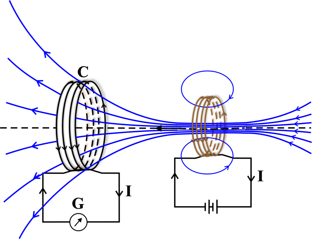
When the second coil is moved towards the first coil, the magnetic flux through the first coil increases. According to Faraday’s second law, this change in flux induces an emf in the first coil, which causes a current to flow in the first coil.
The direction of the current is such that it creates a magnetic field that opposes the increase in flux. This is according to Lenz’s law. The galvanometer pointer shows a deflection, indicating the presence of current in the first coil.
When the second coil is moved away from the first coil, the magnetic flux through the first coil decreases. This also induces an emf in the first coil, which causes a current to flow in the opposite direction. The direction of the current is such that it creates a magnetic field that opposes the decrease in flux. The galvanometer pointer shows a deflection in the opposite direction, indicating the reversal of current in the first coil.
When the second coil is stationary, the magnetic flux through the first coil is constant. This means that there is no change in flux, and hence no induced emf or current in the first coil. The galvanometer pointer shows no deflection, indicating the absence of current in the first coil.
This experiment demonstrates that the relative motion between the two coils produces an induced emf in the first coil, which causes the current to flow. The induced emf is proportional to the rate of change of magnetic flux through the first coil.
Faraday’s Law Derivation
The flux linkage with the coil when the magnet is at position T1 is given by (NΦ1), where (N) is the number of turns in the coil and (Φ1) is the magnetic flux at time T1. Similarly, the flux linkage at time T2 is (NΦ2).
The change in flux linkage between these two times is ( N(Φ2 – Φ1) ). Let’s denote this change in flux linkage as (∆Φ), so:
\(\displaystyle \Delta\Phi = \Phi_2 – \Phi_1 \)
The rate of change of flux linkage over time is given by
\(\displaystyle\frac{N\Delta\Phi}{t} \),
where (t) is the time interval between T1 and T2. Taking the derivative of the flux linkage with respect to time, we get:
\(\displaystyle \frac{d(N\Phi)}{dt} = N \frac{d\Phi}{dt} \)
The equation represents the derivative of the flux linkage with respect to time. Flux linkage (NΦ) is the product of the number of turns in the coil (N) and the magnetic flux (Φ) through one turn of the coil.
Faraday’s Law states that the induced electromotive force (EMF) in a coil is equal to the negative rate of change of the magnetic flux linkage. This is where Lenz’s Law comes into play.
Lenz’s Law tells us that the direction of the induced EMF (and thus the induced current) will be such that it opposes the change in magnetic flux that produced it. This is why we have a negative sign in Faraday’s Law. It’s nature’s way of maintaining balance—induced currents tend to resist the changes in magnetic flux that cause them.
When we combine Faraday’s Law with Lenz’s Law, we get the equation for the induced EMF:
\(\displaystyle \varepsilon = – \frac{d(N\Phi)}{dt} \)
Since (N) is a constant (the number of turns doesn’t change with time), we can take it outside the derivative, which gives us:
\(\displaystyle \varepsilon = -N \frac{d\Phi}{dt} \)
This final equation tells us that the induced EMF in a coil is directly proportional to the negative rate of change of the magnetic flux through the coil. The negative sign is crucial—it ensures that the induced EMF creates a current whose magnetic field opposes the initial change in flux, consistent with Lenz’s Law. So, the transition from the derivative of flux linkage to Faraday’s Law is a direct application of the physical principles of electromagnetic induction and the conservation of energy.
Relationship Between Generated EMF and Flux in Faraday’s Experiment
Michael Faraday’s experiments were crucial in demonstrating the relationship between induced electromotive force (EMF) and magnetic flux.
Faraday’s First Experiment: Faraday connected an ammeter to a loop of wire to measure current. He showed that only when the magnetic field’s intensity changed—as when a magnet was moved towards or away from the loop—did the ammeter register a current. This deflection indicated that an EMF was induced in the wire, which caused the current to flow.
Faraday’s Second Experiment: In another setup, Faraday sent a current through an iron rod, turning it into an electromagnet. He found that relative motion between the magnet and the coil was necessary to induce an EMF. When he rotated the magnet about its axis near the coil, an EMF was induced, but when the magnet was simply spun around its axis without changing its position relative to the coil, no EMF was generated. This highlighted the importance of changing the magnetic field relative to the coil.
Faraday’s Third Experiment: Faraday moved the coil in and out of a stationary magnetic field and observed the galvanometer, which measures small currents. He noted that no current was induced when the coil was stationary relative to the magnetic field. However, when the magnet was moved away from the loop, the ammeter deflected in the opposite direction, indicating that the direction of the induced EMF and thus the current changed with the direction of the magnet’s motion.
These experiments led Faraday to conclude that:
- An EMF is induced in a loop of wire if there is a change in the magnetic flux through the loop.
- The magnitude of the induced EMF is proportional to the rate of change of the magnetic flux.
- The direction of the induced EMF (and thus the current) is such that it opposes the change in magnetic flux that produced it, as stated by Lenz’s Law.
So, Faraday’s experiments show that electricity can be generated by changing magnetic fields, and this principle is used in many applications, from power generation to the functioning of electric motors.
Michael Faraday’s experiments were pivotal in understanding how electric currents can be generated. He demonstrated that a current is produced in a loop of wire when there is a change in the magnetic field around it.
Magnetic flux (Φ) is a measure of the total magnetic field (B) passing through a certain area (A). It’s calculated using the formula:
\(\displaystyle \Phi = B \cdot A \cdot \cos(\theta) \)
where (θ) is the angle between the magnetic field and the perpendicular to the area. The EMF generated in a circuit is directly related to the change in magnetic flux. Faraday found that:
- The EMF is directly proportional to the change in flux (∆Φ).
- The EMF is greatest when the change in time (∆t) is smallest—that is, EMF is inversely proportional to (∆t ).
This relationship is encapsulated in Faraday’s Law of Induction, which states that the magnitude of the induced EMF is proportional to the rate of change of the magnetic flux:
\(\displaystyle \varepsilon = – \frac{d\Phi}{dt} \)
The negative sign indicates that the direction of the induced EMF will oppose the change in magnetic flux, a concept known as Lenz’s Law.
In Faraday’s experiment, when he moved a magnet towards or away from a coil, the magnetic flux through the coil changed, and this change generated an EMF. The faster the magnet moved, the greater the change in flux over a shorter period, resulting in a larger EMF. This is why generators need to rotate quickly to produce a significant amount of electricity.
Also Read: Lenz’s Law
Application of Faraday Law
Faraday’s Law of Electromagnetic Induction has numerous practical applications in our daily lives and various technologies. Here are some key examples:
- Electric Generators: Faraday’s Law is the principle behind the operation of electric generators. When a coil rotates in a magnetic field, it changes the magnetic flux through the coil, inducing an EMF. This is how mechanical energy from wind, water, or steam is converted into electrical energy.
- Transformers: Transformers use Faraday’s Law to change the voltage levels of alternating current (AC). They consist of two coils of wire, known as the primary and secondary coils, wrapped around a magnetic core. A changing current in the primary coil induces a changing magnetic flux in the core, which then induces an EMF in the secondary coil.
- Induction Motors: These motors operate on the principle of electromagnetic induction. When an AC current flows through the stator, it creates a rotating magnetic field, which induces a current in the rotor and causes it to turn.
- Induction Cooking: Induction cooktops have coils beneath the cooking surface. When turned on, they create a magnetic field that induces currents in the pot placed on top, heating it without heating the cooking surface.
- Magnetic Levitation Trains: These trains, also known as maglev trains, use powerful electromagnets that induce currents in the tracks, creating magnetic fields that lift and propel the train forward.
- Electric Guitar Pickups: The strings of an electric guitar are made of a magnetic material. When they vibrate, they change the magnetic flux through the pickup coils, inducing an EMF that is then converted into sound.
These applications show how Faraday’s discovery has been instrumental in advancing technology and improving our quality of life.
Solved Examples
Problem 1: A rectangular loop of wire with dimensions (\(\displaystyle 0.5 \, \text{m} \times 0.2 \, \text{m} \)) is rotating in a uniform magnetic field of (0.1 T). The loop rotates with an angular velocity of (10 rad/s). Calculate the maximum induced EMF in the loop.
Solution: Using Faraday’s Law of Electromagnetic Induction:
\(\displaystyle \mathcal{E} = – \frac{d\Phi}{dt} \)
Magnetic flux (Φ) through the loop:
\(\displaystyle \Phi = B \cdot A \cdot \cos(\omega t) \)
\(\displaystyle \Phi = B \cdot l \cdot w \cdot \cos(\omega t) \)
- (B = 0.1 T)
- (l = 0.5 m)
- (w = 0.2 m)
- (ω = 10 rad/s)
Calculate the area:
\(\displaystyle A = l \cdot w \)
\(\displaystyle A = 0.5 \cdot 0.2\)
\(\displaystyle A = 0.1 \, \text{m}^2 \)
Calculate the induced EMF:
\(\displaystyle \mathcal{E} = – \frac{d}{dt} (B \cdot A \cdot \cos(\omega t)) \)
\(\displaystyle \mathcal{E} = – (B \cdot A \cdot \omega \cdot \sin(\omega t)) \)
Maximum induced EMF occurs when (\(\displaystyle \sin(\omega t) = 1 \)):
\(\displaystyle \mathcal{E}{\text{max}} = B \cdot A \cdot \omega \)
\(\displaystyle \mathcal{E}{\text{max}} = 0.1 \cdot 0.1 \cdot 10 \)
\(\displaystyle \mathcal{E}_{\text{max}} = 0.1 \, \text{V} \)
The maximum induced EMF in the loop is (0.1 V).
Problem 2: A metal rod of length (1 m) moves perpendicularly to a uniform magnetic field of (0.5 T) with a velocity of (2 m/s). Calculate the induced EMF and the induced current if the resistance of the rod is (0.5 ω).
Solution: Using Faraday’s Law:
\(\displaystyle \mathcal{E} = B \cdot l \cdot v \)
Given:
- (B = 0.5 T)
- (l = 1 m)
- (v = 2 m/s)
Calculate the induced EMF:
\(\displaystyle \mathcal{E} = 0.5 \cdot 1 \cdot 2 \)
\(\displaystyle \mathcal{E} = 1 \, \text{V} \)
Calculate the induced current:
\(\displaystyle I = \frac{\mathcal{E}}{R} \)
\(\displaystyle I = \frac{1}{0.5} \)
I = 2 A
The induced EMF is (1 V) and the induced current is (2 A).
Problem 3: A solenoid with (100) turns per meter has a cross-sectional area of (0.01 m2). If the current through the solenoid changes at a rate of (5 A/s), calculate the induced EMF in the solenoid.
Solution: Using Faraday’s Law for a solenoid:
\(\displaystyle \mathcal{E} = -N \frac{d\Phi}{dt} \)
Given:
- Number of turns per meter (n = 100)
- Cross-sectional area (A = 0.01 m2)
- Rate of change of current (\(\displaystyle \frac{dI}{dt} = 5 \, \text{A/s}\) )
Magnetic flux:
\(\displaystyle \Phi = B \cdot A \)
\(\displaystyle B = \mu_0 \cdot n \cdot I \)
\(\displaystyle \frac{d\Phi}{dt} = A \cdot \mu_0 \cdot n \cdot \frac{dI}{dt} \)
Induced EMF:
\(\displaystyle \mathcal{E} = -N \cdot A \cdot \mu_0 \cdot n \cdot \frac{dI}{dt} \)
\(\displaystyle \mathcal{E} = -(100 \cdot 0.01 \cdot 4\pi \times 10^{-7} \cdot 100 \cdot 5) \)
\(\displaystyle \mathcal{E} = -0.628 \, \text{V} \)
The induced EMF in the solenoid is (-0.628 V).
Problem 4: A circular coil of radius (0.2 m) and (50) turns is placed in a uniform magnetic field that changes from (0.2 T) to (0.5 T) in (2 s). Calculate the average induced EMF in the coil.
Solution: Using Faraday’s Law:
\(\displaystyle \mathcal{E} = -N \frac{d\Phi}{dt} \)
Given:
- Number of turns (N = 50)
- Radius (r = 0.2 m)
- Initial magnetic field (Bi = 0.2 T)
- Final magnetic field (Bf = 0.5 T)
- Time (∆t = 2 s)
Area of the coil:
\(\displaystyle A = \pi r^2 \)
\(\displaystyle A = \pi (0.2)^2 \)
\(\displaystyle A = 0.04\pi \, \text{m}^2 \)
Change in magnetic flux:
\(\displaystyle \Delta \Phi = A (B_f – B_i) \)
\(\displaystyle \Delta \Phi = 0.04\pi (0.5 – 0.2) \)
\(\displaystyle \Delta \Phi = 0.04\pi \cdot 0.3 \)
\(\displaystyle \Delta \Phi = 0.012\pi \, \text{Wb} \)
Average induced EMF:
\(\displaystyle \mathcal{E} = -N \frac{\Delta \Phi}{\Delta t} \)
\(\displaystyle \mathcal{E} = -50 \frac{0.012\pi}{2} \)
\(\displaystyle \mathcal{E} = -0.3\pi \)
\(\displaystyle \mathcal{E} \approx -0.942 \, \text{V} \)
The average induced EMF in the coil is approximately (-0.942 V).
Problem 5: A square wire loop of side (0.1 m) is placed in a time-varying magnetic field given by (\(\displaystyle B = 0.02 t \, \text{T} \)), where (t) is in seconds. Calculate the induced EMF at (t = 5 s).
Solution: Using Faraday’s Law:
\(\displaystyle \mathcal{E} = -\frac{d\Phi}{dt} \)
Given:
- Side of the square loop (l = 0.1 m)
- Magnetic field (\(\displaystyle B = 0.02 t \, \text{T} \))
Area of the square loop:
A = l2
A = (0.1)2
A = 0.01 m2
Magnetic flux:
\(\displaystyle \Phi = B \cdot A \)
\(\displaystyle \Phi = 0.02 t \cdot 0.01 \)
\(\displaystyle \Phi = 2 \times 10^{-4} t \)
Induced EMF:
\(\displaystyle \mathcal{E} = -\frac{d\Phi}{dt} \)
\(\displaystyle \mathcal{E} = -\frac{d}{dt} (2 \times 10^{-4} t) \)
\(\displaystyle \mathcal{E} = -2 \times 10^{-4} \)
At (t = 5 s):
\(\displaystyle\mathcal{E} = -2 \times 10^{-4} \)
\(\displaystyle\mathcal{E} = -0.0002 \, \text{V} \)
The induced EMF at (t = 5 s) is ( -0.0002 V).
Problem 6: A coil with (200) turns and a cross-sectional area of (0.05 m2) is placed in a magnetic field that changes from (0.3 T) to (0.7 T) in (0.1 s). Calculate the average induced EMF in the coil.
Solution: Using Faraday’s Law:
\(\displaystyle \mathcal{E} = -N \frac{d\Phi}{dt} \)
Given:
- Number of turns (N = 200)
- Cross-sectional area (A = 0.05m2)
- Initial magnetic field (Bi = 0.3 T)
- Final magnetic field (Bf = 0.7 T)
- Time (∆ t = 0.1 s)
Change in magnetic flux:
\(\displaystyle \Delta \Phi = A (B_f – B_i) \)
\(\displaystyle \Delta \Phi = 0.05 (0.7 – 0.3) \)
\(\displaystyle\Delta \Phi = 0.05 \cdot 0.4 \)
\(\displaystyle \Delta \Phi = 0.02 \, \text{Wb} \)
Average induced EMF:
\(\displaystyle \mathcal{E} = -N \frac{\Delta \Phi}{\Delta t} \)
\(\displaystyle \mathcal{E} = -200 \frac{0.02}{0.1}\)
\(\displaystyle \mathcal{E} = -40 \, \text{V} \)
The average induced EMF in the coil is (-40 V).
FAQs
What is the basic principle behind Faraday’s Laws of Electromagnetic Induction?
Faraday’s Laws of Electromagnetic Induction are based on the principle that a changing magnetic field within a closed loop induces an electromotive force (emf) in the conductor forming the loop. This phenomenon is fundamental to the operation of many electrical devices, such as transformers and electric generators.
What does Faraday’s First Law of Electromagnetic Induction state?
Faraday’s First Law states that an electromotive force (emf) is induced in a conductor when there is a change in the magnetic flux linked with the conductor. In simpler terms, whenever the magnetic environment of a conductor changes, an emf is generated.
What is the significance of Faraday’s Second Law of Electromagnetic Induction?
Faraday’s Second Law quantifies the induced electromotive force (emf) in a conductor. It states that the magnitude of the induced emf is directly proportional to the rate of change of magnetic flux through the conductor. This law helps in calculating the amount of induced voltage based on the change in magnetic flux.
How does Lenz’s Law relate to Faraday’s Laws of Electromagnetic Induction?
Lenz’s Law is a consequence of Faraday’s Law and states that the direction of the induced emf and the resulting current in a closed loop will oppose the change in magnetic flux that produced them. This law ensures the conservation of energy and explains the negative sign in Faraday’s law.
Can you give an example of a practical application of Faraday’s Laws of Electromagnetic Induction?
One practical application of Faraday’s Laws is in electric generators, where mechanical energy is converted into electrical energy. As the generator’s coil rotates within a magnetic field, the change in magnetic flux through the coil induces an emf, generating an electric current.
How does the concept of magnetic flux relate to Faraday’s Laws?
Magnetic flux is a measure of the total magnetic field passing through a given area. In Faraday’s Laws, it is the change in magnetic flux over time that induces an electromotive force (emf) in a conductor. Thus, understanding magnetic flux is crucial for applying Faraday’s Laws to real-world situations.
What role does Faraday’s Law play in the operation of a transformer?
In a transformer, Faraday’s Law is used to transfer electrical energy between two or more coils. A varying current in the primary coil creates a changing magnetic field, which induces an emf in the secondary coil. This induction process allows the transfer of energy and is governed by Faraday’s Laws.