The concept of critical velocity has its roots in fluid dynamics and was developed to understand the behavior of fluid flow in pipes. It’s a fundamental concept that helps predict whether the flow will be smooth (laminar) or chaotic (turbulent).
The concept of critical velocity is deeply rooted in the study of fluid dynamics, a branch of physics that deals with the behavior of fluids (liquids and gases) and their interactions with various forces. The history of critical velocity is particularly tied to the understanding of how fluids flow in different conditions, which is crucial for numerous applications, from engineering to meteorology.
The term “critical velocity” was first introduced in the context of fluid flow through pipes. It was observed that at low speeds, fluids flow in a smooth and orderly manner, known as laminar flow. However, as the speed increases, there comes a point where this orderly flow breaks down into a chaotic and irregular pattern called turbulent flow. The speed at which this transition occurs is what we refer to as the critical velocity.
One of the earliest and most significant contributions to the concept of critical velocity came from Osborne Reynolds, a British engineer and physicist. In 1883, Reynolds conducted experiments to understand the conditions under which laminar flow becomes turbulent. He observed the flow of fluids in pipes and noticed that the nature of the flow changed from laminar to turbulent as the velocity increased. This led to the development of the Reynolds number, a dimensionless quantity that predicts the flow regime in fluid dynamics³.
Reynolds’ work was pivotal because it provided a way to predict the behavior of fluid flow without relying solely on empirical observations. His findings have since become a cornerstone in the field of fluid mechanics, allowing engineers and scientists to design systems that can handle fluids more efficiently and safely.
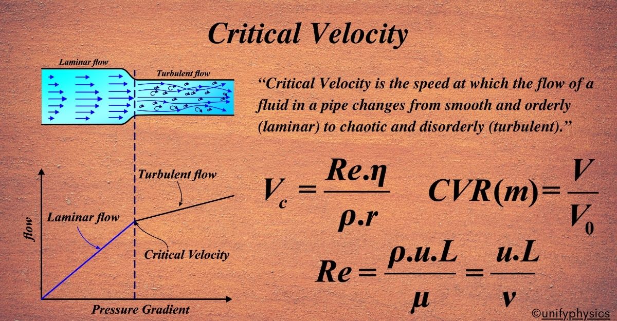
What is Critical Velocity?
Critical Velocity is the speed at which the flow of a fluid in a pipe changes from smooth and orderly (laminar) to chaotic and disorderly (turbulent). It’s a pivotal point in fluid dynamics because it determines the nature of fluid flow.
Imagine you’re watching a river flow. Near the banks, the water moves slowly and smoothly, but in the middle, where the water is faster, it starts swirling and creating whirlpools. This is similar to what happens with critical velocity in fluids.
Critical Velocity is a term used in fluid dynamics to describe the speed at which fluid flow changes from being smooth and straight (laminar) to being chaotic and swirly (turbulent). It’s like the point where the calm river flow suddenly starts to get wild.
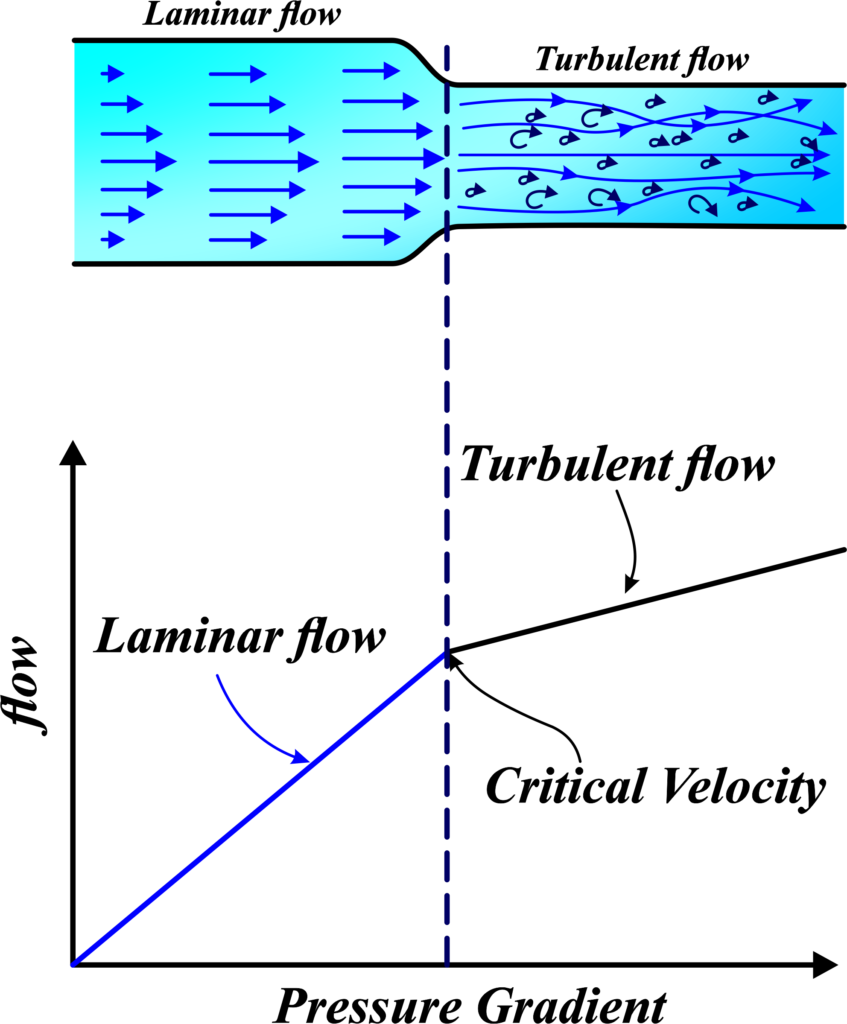
In more technical terms, critical velocity is the threshold speed above which the flow of fluid becomes unpredictable and disorderly. Below this speed, the fluid particles move in an orderly fashion, sliding past each other in straight lines. Above this speed, the particles start moving erratically, bumping into each other and creating a messy flow.
This concept is important because it helps us understand how fluids behave in different situations, like when water flows through pipes or blood flows through arteries. Engineers use this knowledge to design systems that work efficiently, whether it’s for delivering water to our homes or creating medical devices.
So, critical velocity is all about the speed limit for keeping the flow of a fluid nice and orderly. Once you go past this limit, things start to get a bit wild and unpredictable, just like the difference between a peaceful stream and a raging river.
Critical Velocity Formula
When you’re trying to figure out the critical velocity, you’re finding the speed limit for the fluid in the pipe to flow smoothly without causing a ruckus.
To understand the critical velocity formula, let’s think of a water hose. When you open the tap slightly, the water flows out smoothly and in a straight line. This is similar to laminar flow in pipes. But if you open the tap fully, the water gushes out, and the flow becomes chaotic. This is like turbulent flow. The critical velocity is the speed at which the smooth flow turns into a chaotic one.
Now, the formula for critical velocity (Vc) helps us calculate this speed for a fluid flowing through a pipe. It looks like this:
\(\displaystyle\begin{equation}\label{eqn:1}\boxed{\boldsymbol{V_c = \frac{Re \cdot \eta}{\rho \cdot r} }} \end{equation}\)
- (Vc) is the critical velocity, the speed we want to find.
- (Re) is the Reynolds number, which tells us about the flow type (smooth or chaotic).
- (η) is the viscosity of the fluid, which is like the “thickness” or “stickiness” of the fluid.
- (ρ) is the density of the fluid, which is how much mass the fluid has in a certain volume.
- (r) is the radius of the pipe, which is half the diameter of the pipe.
In simple terms, this formula says that the critical velocity depends on how thick the fluid is, how dense it is, and how big the pipe is. If you have a thick fluid (like honey), it will have a higher critical velocity compared to a thin fluid (like water). Similarly, if the pipe is very narrow, the critical velocity will be lower because the fluid can flow smoothly even at higher speeds.
Critical Velocity Dimensional Formula:
When we talk about the dimensional formula of any physical quantity, we’re referring to the way it relates to the basic dimensions of mass (M), length (L), and time (T). For critical velocity, we’re interested in how it can be expressed in terms of these fundamental units. The dimensional formula for critical velocity is given by:
\(\displaystyle [V_c] = M^0L^1T^{-1} \)
The dimensional formula (M0L1T-1) shows that critical velocity has the dimension of length divided by time, which is a way to express speed or velocity. In simpler terms, it’s like saying, “How many meters does something travel in one second?” And that’s exactly what velocity is about – it’s the speed at which the fluid moves.
Critical Velocity Ratio
The critical velocity ratio is not a commonly used term, but it could refer to the ratio of the actual velocity of a fluid to its critical velocity. This ratio helps determine the regime of the flow.
Imagine you’re at a water park, and there’s a slide with water running down it. If the water is moving too slowly, it won’t be fun because you’ll get stuck. If it’s moving too fast, it might wash you away. There’s a sweet spot where the water’s speed is just right for a smooth ride down the slide. This idea is similar to the critical velocity ratio in fluid dynamics.
The Critical Velocity Ratio (CVR) is a way to compare the actual speed of a fluid in a channel or pipe to its critical velocity. The critical velocity is the speed at which the fluid flow changes from smooth (laminar) to chaotic (turbulent).
The CVR is given by the formula:
\(\displaystyle\begin{equation}\label{eqn:2}\boxed{\boldsymbol{ \text{CVR} (m) = \frac{V}{V_o}}} \end{equation}\)
- (m) is the CVR.
- (V) is the mean velocity of the fluid, which is the average speed at which the fluid is moving.
- (Vo) is the critical velocity, the speed above which the flow becomes turbulent.
Now, depending on the value of (m):
- When ( m = 1 ), the flow is perfect, with no silting (where sediment builds up) or scouring (where the pipe gets worn away).
- When ( m > 1 ), the flow is too fast, and scouring will occur.
- When ( m < 1 ), the flow is too slow, and silting will occur.
Also Read: Streamline And Turbulent Flow
Critical Velocity Types
Critical Velocity is further classified into two kinds.
1) Lower Critical Velocity
2) Upper Critical Velocity
Lower Critical Velocity
The lower critical velocity is like the warning sign that tells us, “Hey, the fluid flow is about to get rough, so let’s keep things under control before it gets too wild.”
When we talk about different types of critical velocities, we’re usually referring to the speeds at which the flow of a fluid changes its nature. One of these is the Lower Critical Velocity.
Imagine you’re watching a parade where everyone is marching in a straight, orderly line—that’s like laminar flow in fluids. Now, the lower critical velocity is the speed at which this orderly march starts to get a bit wobbly, and people begin to move out of sync, but they haven’t started running around chaotically yet—that would be turbulent flow.
In technical terms, the lower critical velocity is the speed at which laminar flow (smooth and straight) starts to become unstable. It’s the beginning of the transition period from laminar to turbulent flow. This doesn’t happen suddenly; there’s a range of speeds where the flow is neither completely laminar nor fully turbulent. It’s a bit like the parade marchers starting to shuffle and bump into each other, but they’re not yet in a full-blown scramble.
This concept is important because it helps engineers and scientists predict when a fluid will start to behave unpredictably. By knowing the lower critical velocity, they can design pipes and channels to ensure that the fluid stays in the laminar flow regime for as long as possible, which is usually more efficient and causes less wear and tear on the system.
Upper Critical Velocity
Upper critical velocity is the speed above which you can expect the fluid flow to become a wild ride, full of swirls and eddies, much like a chaotic traffic jam on a highway.
Think of a busy highway where cars are moving smoothly at a steady pace—this is like laminar flow in fluids. Now, the upper critical velocity is like the speed limit above which the traffic starts to get hectic and unpredictable, with cars changing lanes frequently and creating a lot of turbulence.
In fluid dynamics, Upper Critical Velocity refers to the speed at which a fluid’s flow transitions from a transition period (where it’s neither completely laminar nor fully turbulent) to fully turbulent flow. It’s the point where the fluid’s movement becomes highly chaotic, with lots of swirling and mixing.
Here’s a simple way to visualize it:
- Imagine you’re pouring syrup onto a pancake. At first, it flows smoothly in a thin stream (laminar flow). As you pour faster, the stream starts to wobble a bit (transition period). If you pour fast, the syrup splashes and spreads out in all directions (turbulent flow).
- The upper critical velocity is like that moment when you’re pouring so fast that the syrup starts to splash. It’s the threshold where the flow can’t stay smooth anymore and becomes fully turbulent.
Reynolds Number in Critical Velocity Formula
Critical velocity formula, the Reynolds number is used to predict the type of flow we’ll get in a pipe based on the fluid’s properties and the speed it’s moving. It’s a crucial part of the puzzle for figuring out how to keep the flow smooth or when to expect it to get rough.
To understand the Reynolds number, let’s compare it to a game of bowling. When you roll a bowling ball down the lane, it can either go straight (like laminar flow) or it can spin and curve (like turbulent flow). The way the ball moves depends on how fast you roll it and how much spin you put on it.
In fluid dynamics, the Reynolds number is like a score that tells us whether the flow of a fluid in a pipe will be straight and smooth or curvy and chaotic. It’s a dimensionless number, which means it doesn’t have any units like meters or seconds. Instead, it’s just a pure number that comes from a formula. Here’s the formula for the Reynolds number (Re):
\(\displaystyle\begin{equation}\label{eqn:3}\boxed{\boldsymbol{Re = \frac{\rho \cdot u \cdot L}{\mu} = \frac{u \cdot L}{\nu} }} \end{equation}\)
- (ρ) is the density of the fluid—how much stuff is packed into it.
- (u) is the velocity—the speed at which the fluid is moving.
- (L) is a characteristic length—like the diameter of the pipe.
- (µ) is the dynamic viscosity—it’s like the fluid’s thickness or stickiness.
- (ν) is the kinematic viscosity—it’s the dynamic viscosity divided by the density.
Now, when we talk about critical velocity, we’re interested in the speed at which the flow changes from laminar to turbulent. The Reynolds number helps us find that speed. If the Reynolds number is low, the flow is smooth (laminar). If it’s high, the flow gets wild (turbulent).
Critical velocity formula, the Reynolds number is used to predict the type of flow we’ll get in a pipe based on the fluid’s properties and the speed it’s moving. It’s a crucial part of the puzzle for figuring out how to keep the flow smooth or when to expect it to get rough.
Difference between Critical Velocity and Terminal Velocity
Critical Velocity is the threshold speed above which fluid flow becomes turbulent in a pipe. Terminal Velocity is the constant speed that a freely falling object eventually reaches when the resistance of the medium (air, water, etc.) prevents further acceleration.
| Aspect | Critical Velocity | Terminal Velocity |
|---|---|---|
| Definition | The speed at which fluid flow changes from laminar to turbulent in a pipe. | The constant speed that a freely falling object reaches when the force of gravity is balanced by the drag force of the fluid it’s moving through. |
| Occurrence | In fluid dynamics, particularly in enclosed systems like pipes. | In aerodynamics and fluid dynamics, experienced by objects free-falling through a fluid like air or water. |
| Dependence | Depends on factors like fluid density, viscosity, and pipe diameter. | Depends on the object’s mass, surface area, and the density of the fluid it’s falling through. |
| Formula | \(\displaystyle V_c = \frac{Re \cdot \eta}{\rho \cdot r} \) | \(\displaystyle V_t = \sqrt{\frac{2mg}{\rho A C_d}} \) |
| Units | Measured in meters per second (m/s). | Also measured in meters per second (m/s). |
| Relevance | Important for understanding fluid flow in engineering and physics. | Crucial for understanding the motion of falling objects in physics and various applications like parachuting. |
Note:
- (Vt) is terminal velocity,
- (m) is mass,
- (g) is the acceleration due to gravity,
- (ρ) is the fluid density,
- (A) is the cross-sectional area, and
- Cd drag coefficient.
Solved Examples
Example 1: A fluid with a density of (1000 kg/m3) and a viscosity of \(\displaystyle 8.9 \times 10^{-4} \, \text{Pa} \cdot \text{s} \) is flowing through a pipe with a radius of (0.05m). If the Reynolds number at the critical point is (2000), calculate the critical velocity of the fluid in the pipe.
Solution: The critical velocity (Vc) can be calculated using the formula:
\(\displaystyle V_c = \frac{Re \cdot \eta}{\rho \cdot r} \)
Plugging in the values, we get:
\(\displaystyle V_c = \frac{2000 \cdot 8.9 \times 10^{-4}}{1000 \cdot 0.05} \)
\(\displaystyle V_c = \frac{1.78}{50} \)
\(\displaystyle V_c = 0.0356 \, \text{m/s} \)
The critical velocity of the fluid in the pipe is ( 0.0356 m/s).
Example 2: A river with a width of ( 30 m) has a flow rate of ( 90 m3/s). Determine the lower critical velocity for the river if the depth is ( 3m).
Solution: The lower critical velocity (Vlc) can be found by dividing the flow rate by the cross-sectional area of the river:
\(\displaystyle V_{lc} = \frac{Q}{A} \)
The cross-sectional area (A) is the width times the depth:
\(\displaystyle A = w \cdot d \)
\(\displaystyle A = 30 \, \text{m} \cdot 3 \, \text{m} \)
\(\displaystyle A = 90 \, \text{m}^2 \)
Now, calculate the lower critical velocity:
\(\displaystyle V_{lc} = \frac{90 \, \text{m}^3/\text{s}}{90 \, \text{m}^2} \)
\(\displaystyle V_{lc} = 1 \, \text{m/s} \)
The lower critical velocity for the river is ( 1 m/s).
Example 3: A fluid with a kinematic viscosity of \(\displaystyle 1.5 \times 10^{-6} \, \text{m}^2/\text{s} \) is flowing through a pipe with a diameter of (0.1 m). If the upper critical Reynolds number is (4000), find the upper critical velocity.
Solution: The upper critical velocity (Vuc) can be calculated using the Reynolds number formula:
\(\displaystyle Re = \frac{u \cdot D}{\nu} \)
Solving for (u) (upper critical velocity):
\(\displaystyle u = \frac{Re \cdot \nu}{D} \)
Plugging in the values:
\(\displaystyle u = \frac{4000 \cdot 1.5 \times 10^{-6}}{0.1} \)
\(\displaystyle u = \frac{6 \times 10^{-3}}{0.1} \)
\(\displaystyle u = 0.06 \, \text{m/s} \)
The upper critical velocity is ( 0.06 m/s).
Example 4: A pipe has a critical velocity of ( 2 m/s). If the actual velocity of the fluid in the pipe is ( 3 m/s), calculate the critical velocity ratio.
Solution: The critical velocity ratio (m) is given by:
\(\displaystyle m = \frac{V}{V_o} \)
Where (V) is the actual velocity and (Vo) is the critical velocity. Plugging in the values:
\(\displaystyle m = \frac{3}{2} \)
\(\displaystyle m = 1.5 \)
The critical velocity ratio is (1.5).
Example 5: A fluid with a density of ( 900 kg/m3) and a dynamic viscosity of \(\displaystyle 0.001 \, \text{Pa} \cdot \text{s} \) is flowing through a pipe with a diameter of (0.02 m). Calculate the critical velocity if the critical Reynolds number is ( 2300 ).
Solution: First, calculate the kinematic viscosity (ν):
\(\displaystyle \nu = \frac{\mu}{\rho} \)
\(\displaystyle \nu = \frac{0.001}{900} \)
\(\displaystyle \nu = 1.11 \times 10^{-6} \, \text{m}^2/\text{s} \)
Now, use the Reynolds number formula to find the critical velocity (Vc):
\(\displaystyle Re = \frac{V_c \cdot D}{\nu} \)
Solving for (Vc):
\(\displaystyle V_c = \frac{Re \cdot \nu}{D} \)
\(\displaystyle V_c = \frac{2300 \cdot 1.11 \times 10^{-6}}{0.02} \)
\(\displaystyle V_c = \frac{2.553 \times 10^{-3}}{0.02} \)
\(\displaystyle V_c = 0.12765 \, \text{m/s} \)
The critical velocity is ( 0.12765 m/s).
Example 6: A sphere with a radius of ( 0.01 m) and a density of ( 8000 kg/m3) is falling through a fluid with a density of ( 1000 kg/m3 ) and a dynamic viscosity of \(\displaystyle 0.89 \, \text{Pa} \cdot \text{s} \). Calculate the terminal velocity and compare it with the critical velocity if the critical Reynolds number is (2000).
Solution: First, calculate the terminal velocity (Vt) using Stokes’ law for a sphere:
\(\displaystyle V_t = \frac{2gr^2(\rho_s – \rho_f)}{9\mu} \)
Where (ρs) is the density of the sphere, (ρf) is the density of the fluid, and (µ) is the dynamic viscosity. Plugging in the values:
\(\displaystyle V_t = \frac{2 \cdot 9.81 \cdot (0.01)^2 \cdot (8000 – 1000)}{9 \cdot 0.89} \)
\(\displaystyle V_t = \frac{2 \cdot 9.81 \cdot 0.0001 \cdot 7000}{9 \cdot 0.89} \)
\(\displaystyle V_t = \frac{0.1372}{8.01} \)
\(\displaystyle V_t = 0.01715 \, \text{m/s} \)
Now, calculate the critical velocity (Vc) using the Reynolds number formula:
\(\displaystyle V_c = \frac{Re \cdot \nu}{D} \)
First, find the kinematic viscosity (ν):
\(\displaystyle \nu = \frac{\mu}{\rho_f} \)
\(\displaystyle \nu = \frac{0.89}{1000} \)
\(\displaystyle \nu = 8.9 \times 10^{-4} \, \text{m}^2/\text{s} \)
Now, calculate (Vc):
\(\displaystyle V_c = \frac{2000 \cdot 8.9 \times 10^{-4}}{0.02} \)
\(\displaystyle V_c = \frac{1.78}{0.02} \)
\(\displaystyle V_c = 89 \, \text{m/s} \)
The terminal velocity is (0.01715 m/s), and the critical velocity is ( 89 m/s). The terminal velocity is much lower than the critical velocity because the sphere is small and the forces involved are different.
FAQs
What is critical velocity in fluid dynamics, and why is it important?
Critical velocity is the minimum velocity required for a fluid to initiate motion or transition from a state of rest to a state of flow. It’s a crucial parameter in fluid dynamics as it determines whether sediment particles will be entrained or remain stationary in a fluid, influencing processes such as erosion, sediment transport, and river morphology.
What is the difference between lower critical velocity and upper critical velocity?
Lower critical velocity is the minimum velocity required for sediment particles to start moving or be entrained from a stationary state, while upper critical velocity is the maximum velocity beyond which sediment particles are no longer transported and begin to settle or deposit out of the flow.
How are lower and upper critical velocities determined experimentally or analytically?
Lower critical velocity can be determined experimentally by gradually increasing the flow velocity until sediment particles begin to move or be entrained. Upper critical velocity can be determined similarly by gradually decreasing the flow velocity until sediment particles start to settle or deposit out of the flow. Analytically, various equations and models based on sediment transport theory can be used to estimate critical velocities based on factors such as sediment size, density, and flow conditions.
What factors affect the critical velocity of sediment transport in rivers and streams?
The critical velocity of sediment transport is influenced by factors such as sediment size, shape, density, and cohesion, as well as flow velocity, depth, and turbulence. Coarser, heavier, and more irregular sediment particles require higher critical velocities for transport compared to finer, lighter, and more spherical particles.
What is the critical velocity ratio, and how is it calculated or determined?
The critical velocity ratio is the ratio of the actual flow velocity to the critical velocity required for sediment transport. It provides a measure of how close the flow velocity is to the critical velocity and is often used to assess sediment transport potential in rivers and streams. The critical velocity ratio can be calculated by dividing the actual flow velocity by the lower or upper critical velocity, depending on the direction of sediment transport.
How does the critical velocity ratio influence sediment transport and river morphology?
The critical velocity ratio plays a significant role in determining whether sediment will be eroded, transported, or deposited in a river or stream. When the critical velocity ratio is less than one, sediment particles are likely to be entrained and transported downstream, leading to erosion and channel incision. Conversely, when the critical velocity ratio exceeds one, sediment particles are more likely to settle and deposit, leading to aggradation and channel widening.