Electric Field

The story of the electric field begins in the early 19th century with a brilliant scientist named Michael Faraday. Faraday was fascinated by electricity and magnetism, which were relatively new and mysterious forces at the time. He conducted numerous experiments to understand how electric charges interact with each other.

Faraday proposed that charges do not interact directly at a distance, as was previously thought. Instead, he introduced the idea that a charge alters the space around it, creating an “electric field” that extends through the surrounding area. This field then interacts with other charges placed within it.

This was a revolutionary idea because it changed the way scientists thought about force and distance. Before Faraday, the prevailing theory was Coulomb’s law, which stated that electric charges attract or repel each other with a force that is directly proportional to the product of their charges and inversely proportional to the square of the distance between them. While Coulomb’s law could calculate the force between two charges, it didn’t explain how this force could act through empty space.

Faraday’s concept of the electric field filled this gap. It provided a way to visualize and calculate the effect of one charge on another, even if they were not touching. The electric field was a way to map out the influence of a charge at every point in space around it.

Later, James Clerk Maxwell, another giant in the field of physics, built upon Faraday’s ideas. Maxwell developed a set of equations, now known as Maxwell’s equations, which mathematically described how electric and magnetic fields are generated and altered by charges and currents. Maxwell’s equations also predicted the existence of electromagnetic waves, which include visible light, radio waves, and X-rays, among others.

What is an Electric Field?

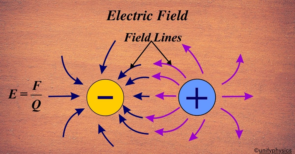
An electric field is a region around a charged particle or object within which a force would be exerted on other charged particles or objects.

Imagine you have a magnet. Even without touching anything, it can pull a paperclip towards itself. This magnet creates an invisible “field” around it that exerts a force on the paperclip. Similarly, charges create an invisible “field” around them that can exert a force on other charges. This is what we call an electric field.

An electric field is essentially the effect that a charged object has on the space around it. It’s like a force field that can push or pull on other charged objects. The strength of this push or pull is what we measure as the electric field strength.

Here’s a simple way to think about it:

• If you place a positive charge somewhere, it creates an electric field around it.
• If you then place another positive charge within that field, it will feel a force pushing it away because like charges repel.
• If the second charge is negative, it will feel a force pulling it towards the first charge because opposite charges attract.

The electric field is a vector field, which means it has both magnitude and direction. The direction of the electric field is always the direction that a positive test charge would move if it were placed in the field.

Electric Field Formula:

The strength of an electric field (E) at a point is defined as the force (F) experienced by a small positive test charge (q) placed at that point divided by the magnitude of the charge:

\(\displaystyle E = \frac{F}{q} \)

• E is the electric field strength at a point.
• F is the force experienced by a test charge placed at that point.
• q is the magnitude of the test charge.

Now, let’s understand this with an analogy. Imagine you’re at a concert and the sound from the speakers is spreading out into the crowd. The sound waves are like the electric field, and the volume you hear is like the force. Just as the volume can be louder near the speakers and quieter farther away, the electric field can be stronger or weaker depending on where you are relative to the charge creating it.

In our formula, E represents how ‘loud’ the electric field is at a point. F is like the ‘volume’ of force you’d feel if you were a positive test charge placed in that field. And q is your ‘volume setting’—the size of the test charge.

The formula tells us that the electric field strength is directly related to the force on the test charge. If the force is high, the electric field is strong. If the force is low, the electric field is weak. It also tells us that the electric field strength is inversely related to the size of the test charge. A larger test charge would ‘hear’ a quieter electric field (feel a smaller force), and a smaller test charge would ‘hear’ a louder electric field (feel a larger force).

It’s important to remember that the test charge should be small so that it doesn’t affect the electric field it’s measuring. Just like if you were measuring the volume of sound, you wouldn’t want your presence to change the sound itself.

Direction Of Electric Field:

The direction of the electric field is determined by the charge creating the field. For a positive charge, the electric field points away from the charge, and for a negative charge, it points towards the charge.

The direction of an electric field is a crucial concept because it tells us how a positive test charge would move if it were placed in the field. To visualize this, let’s use a simple analogy.

Imagine you’re in a field with a bunch of arrows on the ground. These arrows represent the electric field lines. If you were to roll a ball along the ground, you’d naturally roll it in the direction the arrows are pointing. In the same way, if you place a positive test charge in an electric field, it will feel a force that pushes it along the direction of the electric field lines.

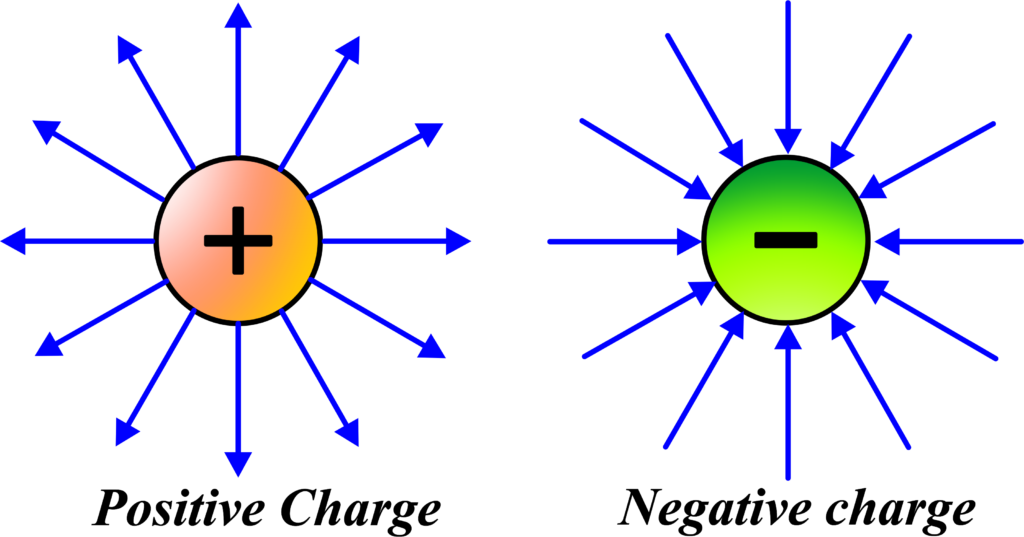
Now, here’s the key point: the electric field lines always point away from positive charges and towards negative charges. So, if you have a positive charge, the electric field lines radiate outwards from it. If you have a negative charge, the electric field lines point inwards towards it. Here’s a simple formula to remember:

• Positive charge: Electric field lines point outwards.
• Negative charge: Electric field lines point inwards.

This means that if you place a positive test charge near another positive charge, it will move away because the electric field tells it to go in that direction. If you place it near a negative charge, it will move towards the negative charge, following the direction of the electric field lines.

In mathematical terms, when we talk about the electric field \(\displaystyle\vec{E}\)and the force \(\displaystyle\vec{F} \), both are vector quantities, which means they have both magnitude and direction. The direction of the electric field is the same as the direction of the force that a positive test charge would experience.

So, in summary, the direction of the electric field is a guide for positive charges, showing them which way to go. It’s like the arrows on the ground telling you which way to roll the ball.

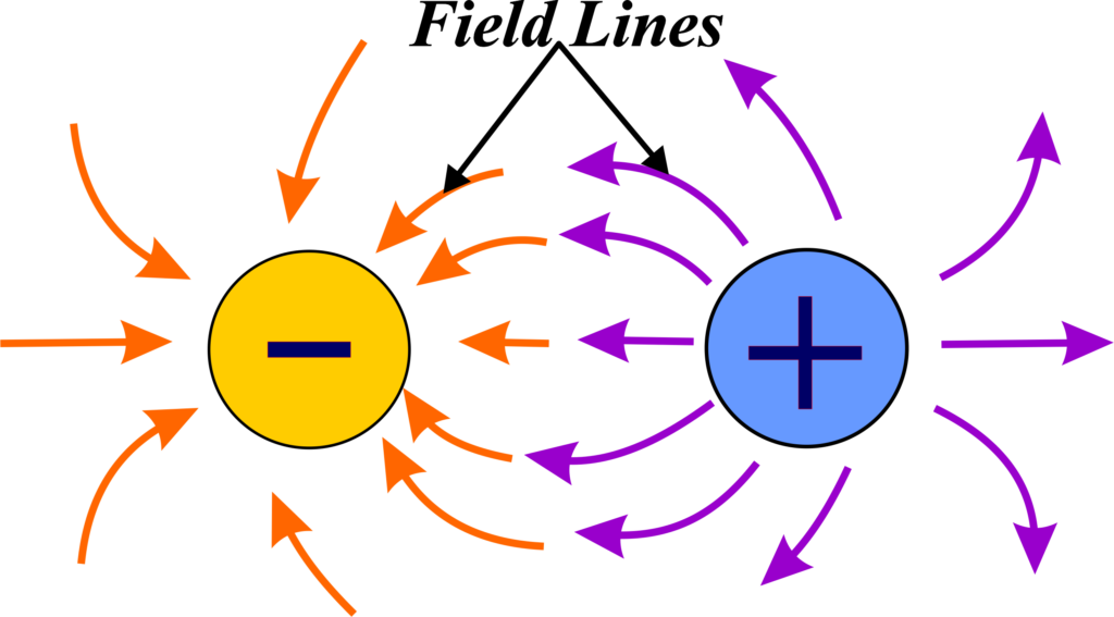
Electric Field Lines

Electric field lines are imaginary lines that represent the direction and strength of the electric field. They radiate out of positive charges and terminate on negative charges.

Electric field lines are like the paths that a positive test charge would follow if it were free to move in the field created by other charges. They are an excellent tool for visualizing electric fields and understanding how charged objects interact with each other.

Electric field lines begin on positive charges and end on negative charges. If there’s only one type of charge, they start or end at infinity. The lines are drawn so that at any point, the tangent to the electric field line matches the direction of the electric field at that point. This means if you place a tiny positive test charge at any point, it will move along the tangent to the field line.

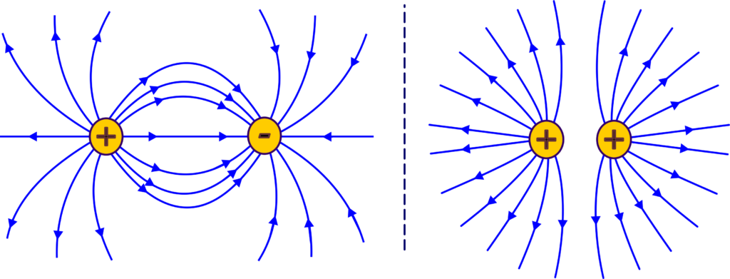
The relative density of field lines around a point corresponds to the relative strength (magnitude) of the electric field at that point. More lines mean a stronger field, and fewer lines mean a weaker field. Electric field lines never intersect each other. If they did, it would imply two different directions for the electric field at that point, which is impossible since electric fields add up vectorially to give a single direction at any point.

The field lines are always perpendicular to the surface of a charged object. This means that if you have a charged sphere, the field lines will radiate outwards or inwards at right angles to the surface.

Let’s use an analogy to make this even clearer. Imagine you’re in a field with a bunch of arrows painted on the ground. These arrows show you the path you should walk along. Now, if the arrows are very close together, that means you’re in a strong wind area—the wind being analogous to the electric field. If the arrows are far apart, the wind is weaker. You can’t walk in two different directions at the same point, which is why the arrows (field lines) never cross. When you reach a hill (a charged object), the arrows will lead you straight up or down the slope (perpendicular to the surface).

Properties of Electric Field Lines

Electric field lines are a visual tool we use to represent how electric fields behave around charges. Here are their key properties:

• Invisible Paths: Think of electric field lines as invisible paths that show how a positive test charge would move if placed in the field.
• Start and End Points: These lines start at positive charges and end at negative charges. If there’s only one type of charge, they start or end at infinity.
• Never Cross: Electric field lines never cross each other. If they did, it would mean a test charge at that point would have two directions to move at the same time, which is impossible.
• Density: The density of the lines indicates the strength of the field. More lines packed together mean a stronger field and lines spread out mean a weaker field.
• Perpendicular: The lines are always perpendicular to the surface of a charged object. This means they make a right angle with the surface.
• Continuous: In a region without any charges, electric field lines are smooth and continuous.
• No Closed Loops: Electric field lines never form closed loops because electric fields are conservative; they don’t have a beginning or an end like a circle would imply.

To help visualize these properties, imagine you’re drawing a map of a magnetic field around a magnet. You’d draw lines going from the north pole to the south pole, without letting them touch or cross. The closer the lines are to the magnet, the stronger the magnetic field. Now, replace the magnet with charges, and you’ve got a pretty good picture of electric field lines!

These properties are not just rules for drawing; they reflect the physical nature of electric fields and how they influence the environment around them.

Continuous Charge Distribution

When we talk about charges, we usually start with the idea of point charges, which are tiny charged particles that we can think of as being located at a single point in space. But in the real world, charges are often spread out over a certain area or volume. This is what we call continuous charge distribution.

Imagine you have a long wire or a big sheet of metal. These objects are too large to be considered as point charges because they have a lot of charges spread out over their length, surface, or volume. So, we use the concept of continuous charge distribution to describe how these charges are spread out.

When we have a continuous charge distribution, we can’t just use simple formulas like we do for point charges. Instead, we have to use calculus to add up (integrate) the effects of all the little bits of charge spread out over the wire, surface, or volume. This lets us calculate things like the electric field or potential at different points in space. There are three main types of continuous charge distribution:

Linear Charge Distribution

The linear charge distribution is a way to describe how charge is spread along a line, and it requires us to use calculus to calculate the resulting electric field. We describe this using a term called linear charge density (λ), which tells us how much charge is there per unit length of the wire.

Imagine you have a long, thin wire that’s charged. Unlike a point charge, which is concentrated at a single point, the charge on this wire is spread out along its length. This is what we call a continuous charge distribution, and when it’s spread out in a line like this, we specifically refer to it as linear charge distribution.

To describe how much charge is on the wire, we use something called linear charge density, denoted by the Greek letter lambda (λ). It tells us the amount of charge per unit length of the wire. Think of it like this: if you had a string of evenly spaced beads, the linear charge density would be how many beads you have per centimeter of string.

The linear charge density (λ) is defined mathematically as:

\(\displaystyle λ = \frac{dq}{dl} \)

where (dq) is a small amount of charge on a tiny segment of the wire with length (dl).

Now, if we want to calculate the electric field created by this charged wire at some point in space, we can’t just use the simple formula for point charges. Instead, we need to add up (integrate) the contributions from each little piece of the wire. For a small segment of charge (dq), the tiny electric field (dE) it creates at a point is given by Coulomb’s law:

\(\displaystyle dE = \frac{k \cdot dq}{r^2} \)

where (k) is Coulomb’s constant and (r) is the distance from the segment to the point where we’re calculating the field. To find the total electric field, we integrate ( dE ) over the entire length of the wire, taking into account the geometry and how ( r ) changes along the wire.

Surface Charge Distribution

This is when charges are spread over a surface, like on a metal plate. We use surface charge density (σ) to describe this, which is the amount of charge per unit area of the surface.

Imagine you have a thin, flat sheet of metal that’s charged. Unlike a point charge, which is concentrated at a single point, the charge on this sheet is spread out over its entire surface. This is what we call surface charge distribution.

To describe how much charge is on the sheet, we use something called surface charge density, denoted by the Greek letter sigma (σ). It tells us the amount of charge per unit area of the sheet. Think of it like this: if you had a bedsheet sprinkled with glitter, the surface charge density would be how much glitter you have per square inch of the bedsheet.

The surface charge density (σ) is defined mathematically as:

\(\displaystyle σ = \frac{dq}{dA} \)

where (dq) is a small amount of charge on a tiny area of the sheet with area (dA).

Volume Charge Distribution

Imagine filling a balloon with tiny, evenly distributed particles that carry an electric charge. This balloon now represents a volume of space where the charge isn’t just on the surface or along a line, but spread throughout the entire volume. This is what we call volume charge distribution.

To quantify the charge spread out in this volume, we use volume charge density, denoted by the Greek letter rho (ρ). It tells us how much charge is present per unit volume. Think of it like the density of a crowd in a room; volume charge density tells us how many charged ‘people’ are in a ‘room’ of space.

The volume charge density (ρ) is defined as:

\(\displaystyle ρ = \frac{dq}{dV} \)

where (dq) is a small amount of charge in a tiny volume element (dV). So, continuous charge distribution is all about understanding how charges are spread out in larger objects and how this affects the electric fields they create.

Calculate the Electric Field Using Coulomb’s Law

Coulomb’s Law in vector form allows us to calculate the force between two point charges considering both magnitude and direction. The law states that the force \(\displaystyle\vec{F} \) between two point charges (q₁) and (q₂) is directly proportional to the product of their charges and inversely proportional to the square of the distance (r) between them, and it acts along the line joining the two charges.

The electric field \(\displaystyle\vec{E} \) at a point in space due to a charge (q) is defined as the force \(\displaystyle\vec{F}\) experienced by a small positive test charge (q₀) placed at that point, divided by the magnitude of the test charge:

\(\displaystyle \vec{E} = \frac{\vec{F}}{q_0} \)

Now, let’s consider two point charges (q₁) and (q₂) separated by a distance (r). According to Coulomb’s Law, the force \(\displaystyle\vec{F} \) on (q₂) due to (q₁) is:

\(\displaystyle \vec{F} = k \cdot \frac{q_1 \cdot q_2}{r^2} \cdot \hat{r} \)

• (k) is Coulomb’s constant (\(\displaystyle 8.99 \times 10^9 ) N·m²/C²\)).
• \(\displaystyle\hat{r}\) is the unit vector pointing from (q₁) to (q₂).

To find the electric field \(\displaystyle\vec{E} \) created by (q₁) at the position of (q₂), we imagine placing a test charge (q₀) at the position of (q₂). The force \(\displaystyle \vec{F}\) on (q₀) due to (q₁) is then:

\(\displaystyle \vec{F} = k \cdot \frac{q_1 \cdot q_0}{r^2} \cdot \hat{r} \)

Using the definition of the electric field, we substitute \(\displaystyle\vec{F}\) in the equation above:

\(\displaystyle \vec{E} = \frac{\vec{F}}{q_0} = \frac{k \cdot \frac{q_1 \cdot q_0}{r^2} \cdot \hat{r}}{q_0} \)

The test charge (q₀) cancels out, leaving us with the vector form of the electric field due to a point charge (q₁):

\(\displaystyle \vec{E} = \frac{k \cdot q_1}{r^2} \cdot \hat{r} \)

This is the electric field at a distance (r) from a point charge (q₁), pointing in the direction of \(\displaystyle \hat{r} \), which is away from (q₁) if it’s positive and towards (q₁) if it’s negative.

So, we’ve derived that the electric field \(\displaystyle\vec{E} \) created by a point charge (q₁) at a distance ( r ) is given by the vector formula:

\(\displaystyle \vec{E} = \frac{k \cdot q_1}{r^2} \cdot \hat{r} \)

This formula allows us to calculate not only the strength but also the direction of the electric field at any point around a charge.

Also Read: Coulomb’s Law

Calculate the Electric Field Using Gauss’s Law

Gauss’s Law relates the electric field to the charge distribution. For a closed surface, the electric flux through the surface is proportional to the charge enclosed.

Gauss’s Law is a powerful tool in electromagnetism that relates the electric flux passing through a closed surface to the charge enclosed by that surface. It’s stated as:

\(\displaystyle \oint \vec{E} \cdot d\vec{A} = \frac{Q_{\text{enc}}}{\epsilon_0} \)

• \(\displaystyle\oint \vec{E} \cdot d\vec{A}\) is the electric flux through a closed surface,
• \(\displaystyle Q_{\text{enc}} \) is the total charge enclosed within the surface,
• \(\displaystyle\epsilon_0 \) is the permittivity of free space.

Let’s consider a spherical surface surrounding a point charge (Q). We want to find the electric field \(\displaystyle\vec{E} \) at a point on this surface.

Because of the spherical symmetry, the electric field at any point on the surface is the same and points radially outward (or inward if (Q) is negative).

The electric flux through the surface is the product of the electric field and the area of the surface. For a sphere of radius (r), the area is \(\displaystyle 4\pi r^2 \). So, the flux is:

\(\displaystyle \Phi = E \cdot 4\pi r^2 \)

Now, we apply Gauss’s Law. The total flux through the surface is equal to the charge enclosed divided by \(\displaystyle\epsilon_0 \):

\(\displaystyle E \cdot 4\pi r^2 = \frac{Q}{\epsilon_0} \)

To find the electric field, we solve for (E):

\(\displaystyle E = \frac{Q}{4\pi \epsilon_0 r^2} \)

This is the magnitude of the electric field at a distance (r) from a point charge (Q), and it points radially away from (Q) if (Q) is positive, and towards (Q) if (Q) is negative.

So, we’ve derived that the electric field (E) created by a point charge (Q) at a distance (r) using Gauss’s Law is:

\(\displaystyle E = \frac{Q}{4\pi \epsilon_0 r^2} \)

This derivation shows how Gauss’s Law simplifies the process of finding electric fields, especially when dealing with symmetrical charge distributions.

Applications of Electric Field

Electric fields are not just a theoretical concept; they have many practical applications in our daily lives and in various technological fields. Here are some key applications:

• Electrostatic Precipitators: These are devices used to clean industrial smoke by removing dust particles. An electric field is used to charge the particles, which are then attracted to plates of the opposite charge, effectively removing them from the air.
• Van de Graaff Generators: These machines are used to generate high voltages and are often seen in science museums demonstrating static electricity. They use a moving belt to accumulate charge and create a strong electric field at the top of a dome, which can cause hair to stand up or create sparks.
• Capacitors: Capacitors are components in electronic circuits that store energy in an electric field. They are used in various devices to regulate power supply, filter signals, and store energy for a short period. The ability of capacitors to store energy is directly related to the electric field between their plates.
• Medical Imaging: Electric fields play a role in medical imaging techniques, such as MRI (Magnetic Resonance Imaging), where they are used in combination with magnetic fields to produce detailed images of the inside of the body.
• Inkjet Printers: Inkjet printers use electric fields to control the direction of tiny droplets of ink. The electric field charges the ink droplets, which are then directed to specific locations on the paper to create an image or text.
• Particle Accelerators: Electric fields are used in particle accelerators to speed up charged particles to high energies. These accelerated particles are then used in various experiments to study the fundamental properties of matter.
• Electrophoresis: This is a laboratory technique used to separate molecules, such as DNA, based on their size and charge. An electric field is applied to move the charged molecules through a gel, allowing for their separation and analysis.
• Touch Screens: Many touch screens work by detecting changes in an electric field. When a finger touches the screen, it alters the electric field, which is detected and translated into a command by the device.
• Light Propagation: The concept of the electric field is also essential for understanding electromagnetic waves, such as light. Starlight and other forms of electromagnetic radiation travel through vast distances of space as oscillating electric and magnetic fields.

Solved Examples

Example 1: A rod of length (L = 1 m) has a uniform linear charge density (λ = 5 × 10^-6C/m). Calculate the electric field at a point (0.5 m) away from the center of the rod along its perpendicular bisector.

Solution: To find the electric field at a point along the perpendicular bisector of the rod, we use the principle of superposition and symmetry. Due to symmetry, the horizontal components of the electric field cancel out, leaving only the vertical components.

Consider an infinitesimal element (dx) at a distance (x) from the center of the rod. The charge of this element is (dq = λdx).

The electric field due to (dq) at the point (P) (0.5 m away from the center) is given by:

\(\displaystyle dE = \frac{1}{4 \pi \epsilon_0} \cdot \frac{dq}{r^2} = \frac{1}{4 \pi \epsilon_0} \cdot \frac{\lambda \, dx}{(x^2 + (0.5)^2)}\)

The vertical component of (dE) is:

\(\displaystyle dE_y = dE \cdot \frac{0.5}{\sqrt{x^2 + (0.5)^2}} = \frac{1}{4 \pi \epsilon_0} \cdot \frac{\lambda \, dx \cdot 0.5}{(x^2 + 0.25)^{3/2}} \)

Integrating from (-0.5) to (0.5) (since the length of the rod is 1 m):

\(\displaystyle E_y = \int_{-0.5}^{0.5} \frac{1}{4 \pi \epsilon_0} \cdot \frac{\lambda \cdot 0.5 \, dx}{(x^2 + 0.25)^{3/2}} \)

\(\displaystyle E_y = \frac{\lambda \cdot 0.5}{4 \pi \epsilon_0} \int_{-0.5}^{0.5} \frac{dx}{(x^2 + 0.25)^{3/2}} \)

Let \(\displaystyle x = 0.5 \tan \theta \), then \(\displaystyle dx = 0.5 \sec^2 \theta \, d\theta \):

\(\displaystyle E_y = \frac{\lambda \cdot 0.5}{4 \pi \epsilon_0} \int_{-\tan^{-1}(1)}^{\tan^{-1}(1)} \frac{0.5 \sec^2 \theta \, d\theta}{(0.25 \sec^2 \theta)^{3/2}} \)

\(\displaystyle E_y = \frac{\lambda}{8 \pi \epsilon_0} \int_{-\frac{\pi}{4}}^{\frac{\pi}{4}} \frac{d\theta}{\cos^2 \theta} \)

\(\displaystyle E_y = \frac{\lambda}{8 \pi \epsilon_0} \cdot [\tan \theta]_{-\frac{\pi}{4}}^{\frac{\pi}{4}} \)

\(\displaystyle E_y = \frac{\lambda}{8 \pi \epsilon_0} \cdot (1 – (-1)) \)

\(\displaystyle E_y = \frac{\lambda}{4 \pi \epsilon_0} \)

Substituting the values:

\(\displaystyle E_y = \frac{5 \times 10^{-6}}{4 \pi \times 8.854 \times 10^{-12}} \)

\(\displaystyle E_y = \frac{5 \times 10^{-6}}{1.112 \times 10^{-10}} \)

\(\displaystyle E_y \approx 4.49 \times 10^4 \, \text{N/C} \)

Therefore, the electric field at a point (0.5 m) away from the center of the rod along its perpendicular bisector is \(\displaystyle 4.49 \times 10^4 \, \text{N/C}\).

Example 2: A disk of radius (R = 0.1 m) carries a uniform surface charge density \(\displaystyle\sigma = 2 \times 10^{-6} \, \text{C/m}^2\). Calculate the electric field at a point (0.2 m) along the axis perpendicular to the center of the disk.

Solution: The electric field along the axis of a uniformly charged disk is given by:

\(\displaystyle E = \frac{\sigma}{2 \epsilon_0} \left( 1 – \frac{z}{\sqrt{z^2 + R^2}} \right) \)

Substituting the values:

\(\displaystyle E = \frac{2 \times 10^{-6}}{2 \times 8.854 \times 10^{-12}} \left( 1 – \frac{0.2}{\sqrt{0.2^2 + 0.1^2}} \right) \)

\(\displaystyle E = \frac{2 \times 10^{-6}}{1.771 \times 10^{-11}} \left( 1 – \frac{0.2}{\sqrt{0.04 + 0.01}} \right) \)

\(\displaystyle E = 1.129 \times 10^5 \left( 1 – \frac{0.2}{\sqrt{0.05}} \right) \)

\(\displaystyle E = 1.129 \times 10^5 \left( 1 – \frac{0.2}{0.2236} \right) \)

\(\displaystyle E = 1.129 \times 10^5 \left( 1 – 0.895 \right) \)

\(\displaystyle E = 1.129 \times 10^5 \times 0.105 \)

\(\displaystyle E \approx 1.186 \times 10^4 \, \text{N/C} \)

Therefore, the electric field at a point (0.2m) along the axis perpendicular to the center of the disk is \(\displaystyle1.186 \times 10^4 \, \text{N/C}\).

Example 3: A ring of radius (R = 0.2 m) carries a uniformly distributed charge \(\displaystyle Q = 1 \, \mu\text{C}\). Calculate the electric field at a point on the axis of the ring, (0.3 m) from its center.

Solution: The electric field on the axis of a uniformly charged ring is given by:

\(\displaystyle E = \frac{1}{4 \pi \epsilon_0} \cdot \frac{Qz}{(R^2 + z^2)^{3/2}} \)

Substituting the values:

\(\displaystyle E = \frac{1 \times 10^{-6} \cdot 0.3}{4 \pi \times 8.854 \times 10^{-12} \cdot (0.2^2 + 0.3^2)^{3/2}} \)

\(\displaystyle E = \frac{3 \times 10^{-7}}{1.112 \times 10^{-10} \cdot (0.04 + 0.09)^{3/2}} \)

\(\displaystyle E = \frac{3 \times 10^{-7}}{1.112 \times 10^{-10} \cdot (0.13)^{3/2}} \)

\(\displaystyle E = \frac{3 \times 10^{-7}}{1.112 \times 10^{-10} \cdot 0.046} \)

\(\displaystyle E = \frac{3 \times 10^{-7}}{5.1152 \times 10^{-12}} \)

\(\displaystyle E \approx 5.86 \times 10^4 \, \text{N/C} \)

Therefore, the electric field at a point on the axis of the ring, (0.3 m) from its center, is \(\displaystyle 5.86 \times 10^4 \, \text{N/C}\).

Example 4: An infinite plane sheet has a uniform surface charge density \(\displaystyle\sigma = 3 \times 10^{-6} \, \text{C/m}^2\). Calculate the electric field near the surface of the sheet.

Solution: The electric field near an infinite plane sheet of charge is given by:

\(\displaystyle E = \frac{\sigma}{2 \epsilon_0} \)

Substituting the values:

\(\displaystyle E = \frac{3 \times 10^{-6}}{2 \times 8.854 \times 10^{-12}} \)

\(\displaystyle E = \frac{3 \times 10^{-6}}{1.771 \times 10^{-11}} \)

\(\displaystyle E = 1.694 \times 10^5 \, \text{N/C} \)

Therefore, the electric field near the surface of the infinite plane sheet is \(\displaystyle1.694 \times 10^5 \, \text{N/C}\).

FAQs