The story of kinematic equations begins in ancient times with the need to understand the motion of celestial bodies. Early astronomers and mathematicians observed the stars and planets, trying to predict their movements. This curiosity laid the groundwork for the field of kinematics.
Kinematics is a term derived from the Greek word “kinesis,” meaning motion. It’s a branch of physics that focuses on the motion of objects without considering the forces that cause this motion. The field can be seen as the “geometry of motion” and is sometimes considered a part of both applied and pure mathematics.
In the 14th century, Nicholas Oresme made significant contributions by representing time and velocity with lengths, inventing a type of coordinate geometry before Descartes. His work helped develop the concept of the derivative, which is fundamental to understanding motion.
The actual kinematic equations that we use today were developed much later. They are based on the work of Galileo Galilei and Sir Isaac Newton. Galileo’s experiments in the late 16th and early 17th centuries led to the discovery that objects accelerate at a constant rate under gravity, regardless of their mass. Later, Newton’s laws of motion, formulated in the 17th century, provided a comprehensive framework for understanding motion and were pivotal in the development of classical mechanics.
In the mid-20th century, further advancements were made. For example, Denavit and Hartenberg introduced a matrix formulation in the 1950s to describe the motion of systems composed of joined parts, like robotic arms or the human skeleton.
These historical milestones have shaped our understanding of motion and the kinematic equations we use today. They allow us to predict moving objects’ positions and have applications in various fields, from engineering to astronomy. By studying these equations, students can gain insight into the fundamental principles that govern movement in our universe. Remember, these equations are not just mathematical expressions; they are the culmination of centuries of human thought and inquiry into the nature of motion.
Uniform Acceleration
In physics, when we talk about acceleration, we’re referring to the rate at which an object’s velocity changes. Now, if this rate of change is constant over time, we call it uniform acceleration. It’s a scenario where, regardless of how much time has passed, the acceleration remains the same. This means that the object’s speed either increases or decreases by the same amount each second.
- Acceleration: It’s a vector quantity, meaning it has both magnitude and direction. It’s defined as the rate of change of velocity with respect to time.
- Uniform: This term implies consistency or sameness. When paired with acceleration, it indicates that the acceleration is unchanging.
Mathematically, uniform acceleration can be expressed as:
\(\displaystyle a = \frac{\Delta v}{\Delta t} \)
where (a) is acceleration, (∆v) is the change in velocity, and (∆t) is the change in time. For uniform acceleration, (a) remains constant.
In the real world, examples of uniform acceleration include a freely falling object under gravity (ignoring air resistance), where the acceleration due to gravity is approximately (9.8 m/s2) downwards, or an elevator moving upwards with a constant increase in speed.
This concept is fundamental because it allows us to use kinematic equations to predict the motion of objects. These equations, which are derived assuming uniform acceleration, help us calculate various aspects of motion, such as displacement, final velocity, and time elapsed.
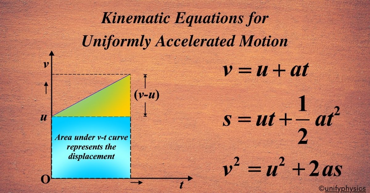
Kinematic Equations for Uniformly Accelerated Motion
These equations describe the motion of an object under uniform acceleration. There are three main equations:
First Kinematic Equation
The first kinematic equation is a fundamental tool in physics that relates an object’s initial velocity, its acceleration, and its final velocity over a certain period of time. It’s expressed as:
\(\displaystyle\begin{equation}\label{eqn:1}\boxed{\boldsymbol{v = u + at }} \end{equation}\)
- (v): Final velocity
- (u): Initial velocity
- (a): Acceleration
- (t): Time
This equation tells us that if we know how fast something is initially moving (u), how much it’s speeding up or slowing down (a), and for how long (t), we can find out its final speed (v).
Think of this equation as a way to predict the future speed of an object based on its current speed and how quickly it’s accelerating. It’s like knowing the pace at which you’re walking and how fast you’re starting to walk faster; with this information, you can figure out how fast you’ll be walking after a certain amount of time.
This equation assumes that the acceleration is constant, meaning it doesn’t change over time. In the real world, this might not always be the case, but it’s a good approximation for many situations, especially in a controlled environment like a physics experiment.
Derivation: Let’s go through the derivation of the first kinematic equation for uniformly accelerated motion, which is a fundamental concept in physics. This equation relates the final velocity of an object to its initial velocity, acceleration, and time of travel.
Acceleration is the rate of change of velocity. It is given by the formula:
\(\displaystyle a = \frac{\Delta v}{\Delta t} \)
When something is moving with constant acceleration, we can find simple equations to connect how far it goes, how long it takes, how fast it started, and how fast it’s going now.
One of these equations is
\(\displaystyle v = u + at \)
This equation helps us figure out how the final velocity of an object relates to its initial velocity and how much it has accelerated over time.
We can rearrange the formula to solve for the final velocity (v):
\(\displaystyle \Delta v = a \Delta t \) \(\displaystyle \hspace{1cm}\text{Since}\) \(\displaystyle \hspace{1cm} (∆ v = v – u )\)
where, (v) is the final velocity and (u) is the initial velocity), we can substitute (∆ v) in the equation:
\(\displaystyle v – u = a \Delta t \)
Adding ( u ) to both sides to isolate ( v ) on one side, we get the first kinematic equation:
\(\displaystyle v = u + a \Delta t \)
This equation tells us that the final velocity (v) of an object is equal to the initial velocity (u) plus the product of the acceleration (a) and the time (∆t) during which the acceleration is applied.
It’s important to note that this derivation assumes that the acceleration is constant, meaning it doesn’t change over the time interval (∆t). This is what we mean by “uniformly accelerated motion.”
Second Kinematic Equation
The second kinematic equation deals with how an object moves when it’s accelerating at a constant rate. This equation is particularly useful because it relates the object’s displacement (how far it has moved) to its initial velocity, acceleration, and time of travel. It’s given by:
\(\displaystyle\begin{equation}\label{eqn:2}\boxed{\boldsymbol{ s = ut + \frac{1}{2}at^2}} \end{equation}\)
Where, (s): Displacement, which is the distance the object has moved in a particular direction.
This equation tells us that if we know an object’s initial speed, how much it’s accelerating, and for how long, we can figure out how far it has traveled. The term \(\displaystyle\frac{1}{2}at^2 \) is particularly important because it shows that the distance an object travels due to acceleration alone is proportional to the square of the time. This means that if you double the time, the distance traveled due to acceleration will be four times as much.
It’s important to note that this equation assumes the acceleration is constant, meaning it doesn’t change over time. This simplification allows us to make accurate predictions about an object’s motion in many situations, even though real-world conditions can sometimes complicate things.
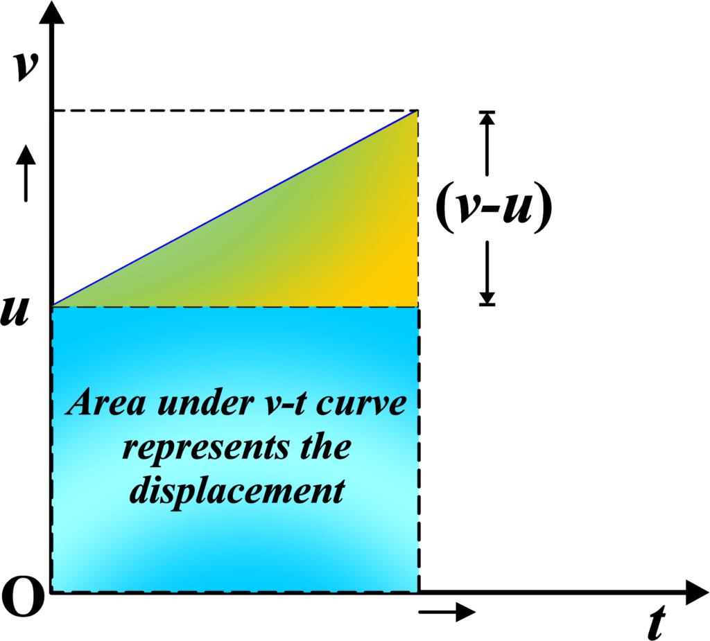
Derivation: The second kinematic equation for uniformly accelerated motion, relates displacement to initial velocity, acceleration, and time.
Average velocity (vavg) is defined as the total displacement (s) divided by the total time (t):
\(\displaystyle v_{avg} = \frac{s}{t} \)
For uniformly accelerated motion, the average velocity is the average of the initial velocity (u) and the final velocity (v). So, we can write:
\(\displaystyle v_{avg} = \frac{u + v}{2} \)
Now, we can equate the two expressions for average velocity:
\(\displaystyle \frac{s}{t} = \frac{u + v}{2} \)
We know from the first kinematic equation that (v = u + at). Let’s substitute (v) in the average velocity equation:
\(\displaystyle \frac{s}{t} = \frac{u + (u + at)}{2} \)
Multiplying both sides by (t) and simplifying, we get:
\(\displaystyle s = \frac{2u + at}{2} \cdot t \)
\(\displaystyle s = ut + \frac{1}{2}at^2 \)
And there we have it, the second kinematic equation:
\(\displaystyle s = ut + \frac{1}{2}at^2 \)
This equation tells us the displacement (s) of an object when it starts with an initial velocity (u), and accelerates uniformly at a rate (a), over a time period (t). It’s a crucial equation for solving problems in kinematics and understanding the motion of objects under uniform acceleration.
Third Kinematic Equation
The third kinematic equation connects an object’s initial velocity, its acceleration, and the displacement it experiences without requiring the final velocity. It’s written as:
\(\displaystyle\begin{equation}\label{eqn:3}\boxed{\boldsymbol{ v^2 = u^2 + 2as}} \end{equation}\)
This equation tells us about the relationship between how fast an object is going initially, how much it’s speeding up, and how far it goes. It’s particularly useful when we don’t know the final velocity but want to find out the distance traveled under constant acceleration.
Imagine you’re pushing a box across the floor. You start slowly (that’s your initial velocity) and then push harder to speed it up (that’s your acceleration). The third kinematic equation helps you figure out how much distance you’ll cover if you keep pushing with the same force.
It’s important to remember that this equation assumes the acceleration is constant, meaning it doesn’t change over the distance or time we’re considering. This makes it a powerful tool for predicting motion in a variety of scenarios, from sliding boxes to launching rockets.
Derivation: The third kinematic equation for uniformly accelerated motion, is a key concept in physics. This equation relates the final velocity squared (v2) to the initial velocity squared (u2), the acceleration (a), and the displacement (s).
Acceleration is the rate of change of velocity. It is given by the formula:
\(\displaystyle a = \frac{\Delta v}{\Delta t} \)
Multiply both sides by (∆t ) to isolate (∆v ):
\(\displaystyle \Delta v = a \Delta t \)
Since (∆v = v – u ) (where (v) is the final velocity and (u) is the initial velocity), we can substitute (∆v ) in the equation:
\(\displaystyle v – u = a \Delta t \)
Adding (u) to both sides to isolate (v) on one side, we get:
\(\displaystyle v = u + a \Delta t \hspace{1cm}\) (i)
Displacement (s) during uniformly accelerated motion can be expressed using the average velocity (vavg) and the time (∆t):
\(\displaystyle s = v_{avg} \Delta t \)
For uniformly accelerated motion, the average velocity is the average of the initial and final velocities:
\(\displaystyle v_{avg} = \frac{u + v}{2} \)
Substitute (vavg) in the displacement equation:
\(\displaystyle s = \left(\frac{u + v}{2}\right) \Delta t \)
Replace (v) with (u + a∆t ) in the displacement equation:
\(\displaystyle s = \left(\frac{u + (u + a \Delta t)}{2}\right) \Delta t \)
Expand and simplify the equation:
\(\displaystyle s = \left(\frac{2u + a \Delta t}{2}\right) \Delta t \)
\(\displaystyle s = u \Delta t + \frac{1}{2} a (\Delta t)^2 \hspace{1cm}\)(ii)
We know from eq.(i) that (v = u + a ∆t). Squaring both sides of this equation gives us:
\(\displaystyle v^2 = (u + a \Delta t)^2 \)
\(\displaystyle v^2 = u^2 + 2u(a \Delta t) + (a \Delta t)^2 \)
From (ii), we see that (u∆t) is part of the expression for (s), so we can write:
\(\displaystyle s = u \Delta t + \frac{1}{2} a (\Delta t)^2 \hspace{1cm}\) as: \(\displaystyle \hspace{1cm} 2u \Delta t = 2s – a (\Delta t)^2 \)
Substitute (2u∆t) back into the equation for (v2):
\(\displaystyle v^2 = u^2 + 2s – a (\Delta t)^2 + (a \Delta t)^2 \)
The terms (a∆t2) cancel each other out, leaving us with:
\(\displaystyle v^2 = u^2 + 2as \)
And there we have it, the third kinematic equation:
\(\displaystyle\begin{equation}\label{eqn:6}\boxed{\boldsymbol{ v^2 = u^2 + 2as}} \end{equation}\)
This equation is very useful for solving problems where you need to find the final velocity of an object when its initial velocity, acceleration, and displacement are known.
Also Read: Acceleration
Uniformly Accelerated Motion In Plane
When we talk about motion in a plane, we often refer to projectile motion as a common example. In projectile motion, an object is thrown with an initial velocity at an angle into the air, and the only acceleration it experiences is due to gravity (g), acting downwards.

In uniformly accelerated motion in a plane, we’re dealing with motion that occurs in two dimensions. This is a step up from motion along a straight line because now we have to consider two directions, such as horizontal and vertical.
Uniform acceleration in a plane still means that the object’s velocity is changing at a constant rate, but now this change can happen in more than one direction. For example, when you throw a ball, it moves both forward and upward at the same time.
The most common example of uniformly accelerated motion in a plane is projectile motion. When you throw a ball at an angle, it follows a curved path. This happens because of two things:
- The ball moves horizontally with a constant velocity (because there’s no acceleration in the horizontal direction if we ignore air resistance).
- At the same time, the ball accelerates vertically due to gravity, which pulls it down toward the ground.
So, in projectile motion, the only acceleration acting on the object is due to gravity (usually denoted as ‘g’), and it’s always directed downwards. This means that while the horizontal component of the ball’s velocity remains constant, the vertical component changes uniformly over time.
To analyze such motion, we use the kinematic equations separately for the horizontal (x-direction) and vertical (y-direction) components of motion.
Horizontal Motion: When we talk about motion in a plane, we’re referring to movement in two dimensions. For horizontal motion under uniform acceleration, we’re specifically looking at how an object moves along a straight path in a horizontal direction when it’s experiencing constant acceleration.
- Uniform Acceleration: This means the object’s speed is changing at a constant rate. In horizontal motion, this could be due to a force being applied in the horizontal direction, like a car accelerating on a road.
- Horizontal Plane: This is a flat, level surface extending in all directions. In our case, it’s the direction in which the object is moving without any vertical displacement.
- No Vertical Acceleration: Typically, in horizontal motion, we assume there’s no vertical acceleration affecting the object, meaning gravity isn’t pulling it down or up as it moves forward.
In the horizontal direction, if we assume there’s no resistance (like air resistance), then the object would continue to move with uniform acceleration. The kinematic equations for horizontal motion are similar to those in one dimension, but they only consider the horizontal component of the motion. The basic equation for horizontal motion with uniform acceleration is:
\(\displaystyle v = u + at \)
For displacement in the horizontal direction, we use:
\(\displaystyle s = ut + \frac{1}{2}at^2 \)
where (s) is the horizontal displacement.
Imagine sliding a hockey puck on an air hockey table. If you give it a push, it will slide across the table with a constant acceleration until it either hits the side or is stopped. If you were to push it harder, the acceleration would be greater, and it would reach the other side faster.
Vertical Motion: When we analyze motion in a plane, we consider both horizontal and vertical components. For vertical motion, the concept of uniform acceleration is often demonstrated through the example of gravity acting on objects.
- Vertical Motion: This refers to the movement of an object up or down in a vertical plane.
- Uniform Acceleration: In the context of vertical motion, this usually refers to the constant acceleration due to gravity, denoted as (g), which is approximately (9.8 m/s2 ) near the Earth’s surface.
- Direction: The direction of acceleration due to gravity is always downwards, towards the center of the Earth.
The kinematic equations for vertical motion with uniform acceleration are similar to those for one-dimensional motion, but they specifically apply to the vertical component of motion. The basic equation for vertical motion with uniform acceleration is:
\(\displaystyle\begin{equation}\label{eqn:4}\boxed{\boldsymbol{v = u + gt}} \end{equation}\)
For displacement in the vertical direction, we use:
\(\displaystyle\begin{equation}\label{eqn:5}\boxed{\boldsymbol{s = ut + \frac{1}{2}gt^2 }} \end{equation}\)
Consider an object being thrown upwards. As it rises, it slows down due to gravity pulling it back down, until it momentarily stops at its highest point. Then, it begins to fall back down, accelerating due to gravity. Throughout this motion, the acceleration remains constant at (g), but the velocity changes direction from upward to downward.
This concept is crucial for understanding phenomena like projectile motion, where an object has both a horizontal velocity (which remains constant if we ignore air resistance) and a vertical velocity (which changes due to gravity). By mastering the equations and concepts of vertical motion, students can predict the behavior of objects thrown or dropped, calculate their maximum height, and determine the time they take to land. It’s a fundamental aspect of kinematics that has real-world applications in sports, engineering, and many other fields.
By combining these two motions, we can predict the entire path of the projectile. This concept is not only fascinating but also incredibly useful in various fields, from sports to space science. Understanding uniformly accelerated motion in a plane allows students to grasp the complexities of real-world motion and lays the foundation for more advanced physics concepts.
Solved Examples
Problem 1: A car starts from rest and accelerates uniformly at (3 m/s2) for (10) seconds. What is its final velocity?
Solution: Using the kinematic equation:
\(\displaystyle v = u + at \)
where (u) is the initial velocity, (a) is the acceleration, and (t) is the time.
Given:
\(\displaystyle u = 0 \, \text{m/s} \)
\(\displaystyle a = 3 \, \text{m/s}^2 \)
t = 10 s
\(\displaystyle v = 0 + (3 \times 10) \)
\(\displaystyle v = 30 \, \text{m/s} \)
The final velocity of the car is (30 m/s).
Problem 2: A train accelerates uniformly from rest at (2 m/s2 ) for (8) seconds. Calculate the distance it travels during this time.
Solution: Using the kinematic equation:
\(\displaystyle s = ut + \frac{1}{2}at^2 \)
Given: u = 0 m/s; a = 2 m/s2; t = 8 s.
\(\displaystyle s = (0 \times 8) + \frac{1}{2} (2 \times 8^2) \)
\(\displaystyle s = 0 + \frac{1}{2} (2 \times 64) \)
\(\displaystyle s = \frac{1}{2} \times 128 \)
s = 64 m
The train travels (64 m) during this time.
Problem 3: A car initially moving at (5 m/s) accelerates uniformly at (4 m/s2). How long will it take to reach a velocity of (25 m/s)?
Solution: Using the kinematic equation:
v = u + at
Given: u = 5 m/s; v = 25 m/s; a = 4 m/s2
Rearrange the equation to solve for (t):
\(\displaystyle t = \frac{v – u}{a} \)
\(\displaystyle t = \frac{25 – 5}{4} \)
\(\displaystyle t = \frac{20}{4} \)
t = 5 s
It will take (5 s) to reach a velocity of (25 m/s).
Problem 4: A projectile is launched with an initial velocity of (50 m/s) at an angle of (30∘) to the horizontal. Calculate the range and maximum height of the projectile.
Solution: First, decompose the initial velocity:
\(\displaystyle u_x = u \cos \theta = 50 \cos 30^\circ = 50 \times \frac{\sqrt{3}}{2} = 25\sqrt{3} \, \text{m/s} \)
\(\displaystyle u_y = u \sin \theta = 50 \sin 30^\circ = 50 \times \frac{1}{2} = 25 \, \text{m/s} \)
Time of flight:
\(\displaystyle T = \frac{2u_y}{g} = \frac{2 \times 25}{9.8} \approx 5.10 \, \text{s} \)
Range:
\(\displaystyle R = u_x \times T = 25\sqrt{3} \times 5.10 \approx 220.96 \, \text{m} \)
Maximum height:
\(\displaystyle H = \frac{u_y^2}{2g} = \frac{25^2}{2 \times 9.8} \approx 31.89 \, \text{m} \)
The range of the projectile is approximately (220.96 m) and the maximum height is approximately (31.89 m).
Problem 5: A ball is thrown vertically upward with a velocity of (20 m/s). Calculate the time to reach the highest point and the maximum height reached.
Solution: To reach the highest point, the final velocity (v) is (0).
Using the kinematic equation:
v = u + at
Given: u = 20 m/s; a = -9.8 m/s2; v = 0
0 = 20 + (-9.8)t
9.8t = 20
\(\displaystyle t = \frac{20}{9.8} \approx 2.04 \, \text{s} \)
Maximum height:
\(\displaystyle s = ut + \frac{1}{2}at^2 \)
\(\displaystyle s = 20 \times 2.04 + \frac{1}{2} (-9.8) (2.04)^2 \)
\(\displaystyle s \approx 40.8 – 20.39 \)
\(\displaystyle s \approx 20.41 \, \text{m} \)
The time to reach the highest point is approximately (2.04 s) and the maximum height is approximately (20.41 m).
Problem 6: A particle moves in a plane with uniform acceleration. Its initial velocity is (5 m/s) in the (x)-direction and it accelerates uniformly at (2 m/s2) in the (y)-direction. Calculate its displacement after (3) seconds.
Solution: Initial velocity components:
\(\displaystyle u_x = 5 \, \text{m/s} \)
\(\displaystyle u_y = 0 \, \text{m/s} \)
Acceleration components:
ax = 0
\(\displaystyle a_y = 2 \, \text{m/s}^2 \)
Displacement in (x)-direction:
\(\displaystyle s_x = u_x t + \frac{1}{2} a_x t^2 \)
\(\displaystyle s_x = 5 \times 3 + \frac{1}{2} \times 0 \times 3^2 \)
sx = 15 m
Displacement in (y)-direction:
\(\displaystyle s_y = u_y t + \frac{1}{2} a_y t^2 \)
\(\displaystyle s_y = 0 \times 3 + \frac{1}{2} \times 2 \times 3^2 \)
\(\displaystyle s_y = 0 + \frac{1}{2} \times 2 \times 9 \)
\(\displaystyle s_y = 9 \, \text{m} \)
Resultant displacement:
\(\displaystyle s = \sqrt{s_x^2 + s_y^2} \)
\(\displaystyle s = \sqrt{15^2 + 9^2} \)
\(\displaystyle s = \sqrt{225 + 81} \)
\(\displaystyle s = \sqrt{306} \)
\(\displaystyle s \approx 17.49 \, \text{m} \)
The displacement after (3) seconds is approximately (17.49 m).
FAQs
What exactly is uniformly accelerated motion?
Uniformly accelerated motion refers to motion where an object experiences a constant acceleration, meaning its velocity changes at a steady rate over time. This type of motion is described by kinematic equations that predict the object’s position and velocity at any given time.
Can we use the kinematic equations if the acceleration is not constant?
The kinematic equations are specifically derived for uniformly accelerated motion, where acceleration remains constant. If acceleration varies with time, these equations may not provide accurate results. However, for small time intervals or when the variation in acceleration is negligible, the kinematic equations can still offer useful approximations.
How do we derive the kinematic equations for uniformly accelerated motion?
The kinematic equations can be derived using calculus and the fundamental principles of motion. By integrating the equations of motion with respect to time and applying appropriate initial conditions, we can derive these equations, which describe the relationships between displacement, velocity, acceleration, and time for uniformly accelerated motion.
How do the kinematic equations help in solving real-world problems?
The kinematic equations provide a systematic approach to solving motion problems by relating the initial and final conditions of motion to the time elapsed and the acceleration experienced. They allow us to predict an object’s position, velocity, and acceleration at any given time, making them invaluable tools in various fields, including engineering, physics, and astronomy.
Can the kinematic equations be used in scenarios involving negative acceleration?
Yes, the kinematic equations are applicable in scenarios where the acceleration is negative, indicating deceleration or motion in the opposite direction of the initial velocity. In such cases, the negative sign is simply incorporated into the acceleration term in the equations.
Are there any limitations to using the kinematic equations?
While the kinematic equations are powerful tools for solving motion problems, they have limitations, particularly when dealing with non-uniform acceleration, relativistic speeds, or situations involving complex forces. In such cases, more advanced mathematical techniques or physical principles may be necessary for accurate predictions.
How do we verify the accuracy of solutions obtained using the kinematic equations?
Solutions obtained using the kinematic equations can be verified through experimental observations or by comparing them with results obtained using alternative methods, such as numerical simulations or theoretical analyses. Consistency between predicted and observed outcomes confirms the accuracy of the solutions.
Can the kinematic equations be used to describe rotational motion?
No, the kinematic equations are formulated specifically for translational motion along a straight line and do not apply to rotational motion. For rotational motion, different sets of equations, such as those derived from rotational dynamics or rigid body kinematics, are used to describe the relationships between angular displacement, angular velocity, angular acceleration, and time.