
The concepts of scalars and vectors are deeply rooted in the history of mathematics and physics. They are essential tools that scientists and mathematicians use to describe the world around us.
Scalars have been around since the early days of algebra, where simple numbers represented quantities like distance, mass, and time. These are quantities that have magnitude but no direction.
Vectors, however, are a bit more complex. They emerged from the need to represent physical quantities that have both magnitude and direction, such as force and velocity. The idea of vectors is intuitive; for example, it’s not enough to say that a car is moving at 60 km/h. We also need to know the direction of its movement to get the complete picture.
The modern mathematical treatment of vectors began in the 19th century. William Rowan Hamilton introduced the term “vector” itself as he worked on complex numbers and quaternions. He used vectors to represent quantities in three-dimensional space.
The parallelogram law for vector addition, which is a cornerstone of vector mathematics, has an even older history. It may have appeared in the lost works of Aristotle and was certainly known by the time of Isaac Newton, who used it in his seminal work, “Principia Mathematica.”
In the 20th century, vectors became even more important with the development of vector spaces in linear algebra, which now form the basis for much of modern physics and engineering.
What Is a Scalar Quantity?
A scalar quantity is defined by only its magnitude (size or amount) and has no direction. A scalar quantity in physics is a physical quantity that has magnitude but no specific direction associated with it. In simpler terms, we can measure it with a single number, but we don’t need to know which way it’s pointing.
Properties
- Magnitude: Scalar quantities only have magnitude, which means they represent the size or amount of something. For example, if you have a mass of 5 kilograms, the “5” represents the magnitude of the mass.
- No Direction: Unlike vector quantities (which we’ll discuss later), scalar quantities do not have a specific direction associated with them. This means they are fully described by their magnitude alone.
- Additive: Scalar quantities can be added together algebraically, regardless of their direction. For example, if you’re driving at 50 kilometers per hour and then speed up to 60 kilometers per hour, your total speed is the sum of the two scalar quantities:
50+60=110 kilometers per hour.
Imagine you’re baking a cake. You need certain ingredients like flour, sugar, and eggs. Each of these ingredients is measured by just how much you need—like 2 cups of flour, 1 cup of sugar, and 3 eggs. You don’t need to specify a direction to add them to your mix, right? In physics, quantities like these are called scalars.
A scalar quantity is something that is completely described by its magnitude alone. The magnitude is just a fancy term for the size or amount of something. Scalars don’t care about direction; they’re all about how much there is of something. For example:
- Time: It just flows on. We measure it in seconds, minutes, or hours, but we never say time is moving “north” or “to the left.”
- Temperature: It tells us how hot or cold something is, measured in degrees Celsius or Fahrenheit, but not in which direction the heat is going.
- Mass: It’s how much matter is in an object, measured in kilograms or pounds, but mass doesn’t have a direction.
So, when you’re dealing with scalars, remember, it’s all about the amount. No need to worry about where it’s going or coming from. It’s like the score in a game—what matters is how many points you have, not where on the scoreboard they are.
Scalars are the straightforward, no-nonsense numbers in physics that tell us how much of something we have, without any fuss about directions. They’re the simple ingredients in the recipe for understanding the universe!
What Is a Vector Quantity?
In contrast, a vector quantity has both magnitude and direction. A vector quantity in physics is a physical quantity that has both magnitude and direction. In simpler terms, we can measure it with both a number and an arrow indicating which way it’s pointing.
Properties
- Magnitude: Like scalar quantities, vector quantities have magnitude, which represents the size or amount of the quantity being measured. For example, if you’re measuring velocity, the magnitude might be 50 kilometers per hour.
- Direction: What sets vector quantities apart is that they also have direction. This direction is indicated by an arrow, which shows which way the quantity is pointing. For example, if you’re measuring velocity, the arrow might indicate that you’re moving north at 50 kilometers per hour.
- Components: Vector quantities can be broken down into components along different axes. For example, if you have a velocity vector pointing northeast, you can break it down into its northward and eastward components.
Think of a vector quantity as a travel direction. It’s not enough to say you’re going 60 km/h; you need to know where you’re headed—like 60 km/h north. That’s what vectors are all about magnitude and direction.
A vector quantity is something that is described by both how much there is of something (magnitude) and where it’s going (direction). Here are some examples:
- Velocity: It’s not just how fast you’re going, but also in which direction. So, if you’re driving at 50 km/h east, that’s a vector.
- Force: When you push something, you apply force in a specific direction. That’s why force is a vector; it has both strength (magnitude) and direction.
- Acceleration: It tells us how quickly velocity is changing and in which direction, making it a vector too.
Representing Vectors
Vectors are usually represented by arrows. The length of the arrow shows the magnitude, and the arrow points in the direction of the vector. For example, an arrow pointing upwards with a certain length could represent a force of 10 N pushing upwards.
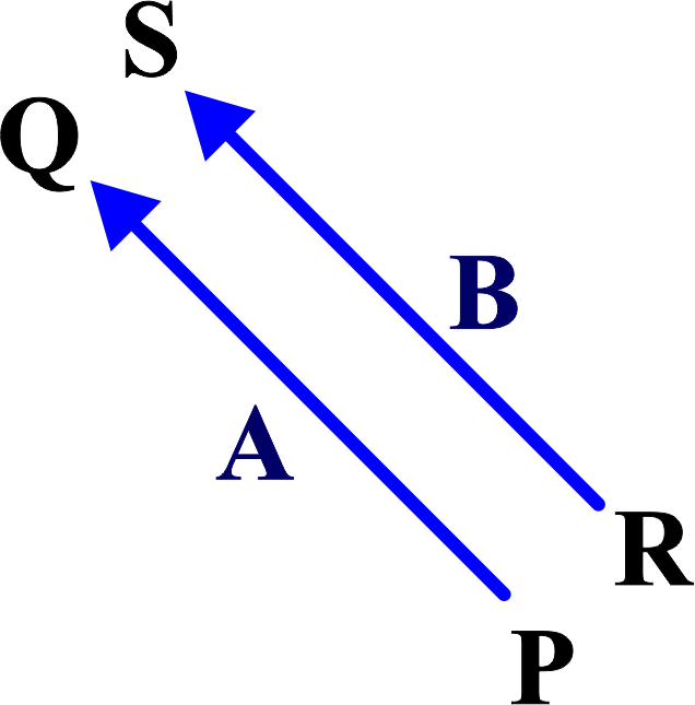
Imagine you have two identical arrows, A and B. If you want to check if they’re the same.
Take one arrow, let’s say B, and move it next to the other arrow, A. Shift B without turning it until its starting point lines up with A’s starting point. Now, if the tips of both arrows are in the same spot, we can say they’re equal. So, if the tips of arrows A and B match up, we know they’re the same length and direction.
Vectors are crucial because they let us accurately describe movements and forces in the real world. Without direction, we’d have no way to control or predict where things will end up!
So, when you’re dealing with vectors, remember, it’s like giving someone directions. You need to tell them both how far to go and where to turn. That’s what makes vectors so powerful in physics—they give us the complete picture.
Vector Notation
When we talk about vectors, we’re talking about quantities that have both a size and a direction. To communicate this information clearly, we use vector notation. Vectors are typically represented by an arrow. The length of the arrow indicates the magnitude, and the direction of the arrow shows the direction of the vector.
How to Write Vectors: Vectors are usually written with an arrow over a letter, like this: \(\displaystyle \vec{v} \) or \(\displaystyle\vec{F} \). This tells us that we’re not just dealing with a regular number (scalar), but with something that points in a specific direction.
In diagrams, vectors are represented by arrows. The length of the arrow shows how big the vector is (its magnitude), and the direction of the arrow shows where the vector is pointing.
Components of Vectors: Sometimes, we need to be more specific about where a vector is pointing, especially in 3D space. We can break down a vector into its components along the x, y, and z axes. For example, a vector \(\displaystyle\vec{v}\) might be written in component form as (vx, vy, vz), where (vx), (vy), and (vz) are the magnitudes of the vector in the direction of each axis.
Unit Vectors: We also have special vectors called unit vectors that have a magnitude of 1 and point along the axes of our coordinate system. These are usually denoted by \(\displaystyle\hat{i}\), \(\displaystyle\hat{j} \), and \(\displaystyle\hat{k}\) for the x, y, and z directions, respectively.
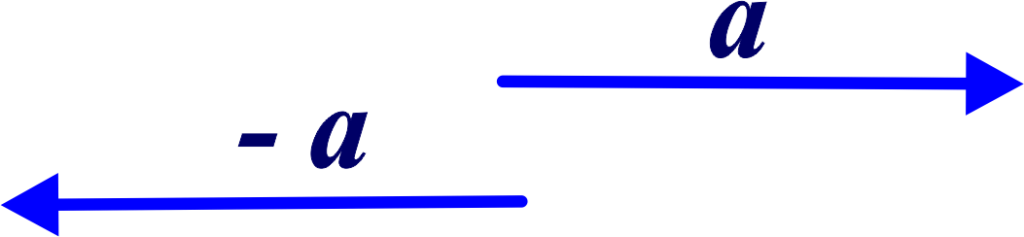
Negative Vectors: If a vector points in the opposite direction, we can denote it with a negative sign.
So, if \(\displaystyle \vec{a} \) is a vector pointing to the right, \(\displaystyle -\vec{a} \) would be the same vector but pointing to the left.
Adding Vectors: When we add vectors, we’re combining their magnitudes and directions. If two vectors are going in the same direction, we just add their magnitudes. If they’re going in opposite directions, we subtract one from the other.
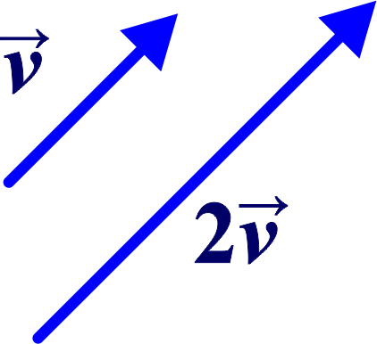
Scalar Multiplication: When we multiply a vector by a scalar (a regular number), we’re changing its magnitude but not its direction. So if we have a vector \(\displaystyle\vec{v} \) and we multiply it by 2, the new vector \(\displaystyle 2\vec{v} \) will be twice as long but point in the same direction.
By using vector notation, we can precisely describe quantities that move and interact in space, which is essential for solving problems in physics.
Difference Between Scalars and Vectors
The key difference is that scalars do not have direction, while vectors do. This means that vector quantities can cancel each other out or add up depending on their direction, unlike scalars.
| Aspect | Scalar Quantities | Vector Quantities |
|---|---|---|
| Definition | Scalars are quantities that are fully described by a magnitude (or numerical value) alone. | Vectors are quantities that are described by both a magnitude and a direction. |
| Direction | Scalars do not have direction. | Vectors have a specific direction. |
| Examples | Temperature, Mass, Time, Speed, Energy | Velocity, Displacement, Force, Acceleration, Momentum |
| Addition | Scalars add algebraically. For example, 3 kg + 2 kg = 5 kg. | Vectors add geometrically, following rules like the triangle law or parallelogram law. |
| Symbol Representation | Usually denoted by italicized or plain letters e.g.,(s), (m), (t). | Represented by boldfaced letters or letters with an arrow on top e.g.,\(\displaystyle \mathbf{v}\),\(\displaystyle\vec{F}\). |
| Multiplication | Scalars multiply like ordinary numbers. For example, doubling the mass: \(\displaystyle 2 \times 3 \text{ kg} = 6 \text{ kg}\). | Multiplying a vector by a scalar changes its magnitude but not its direction. For example, doubling the force in the same direction: \(\displaystyle 2 \times \vec{F} \). |
| Zero Value | Zero scalar has a clear meaning (e.g., zero temperature). | Zero vector \(\displaystyle( \vec{0} )\) has a magnitude of zero but no specific direction. |
| Physical Significance | Scalars often represent the ‘amount’ of a physical quantity. | Vectors represent quantities that have a ‘direction’ in space and are essential in describing motion and forces. |
Position and Displacement Vectors
A position vector describes the position of a point in space relative to an origin, while a displacement vector represents the change in position of an object.
Position Vectors
Position vectors are like addresses in the universe. They tell us where an object is located in space relative to a chosen reference point, usually called the origin. Just as your home address pinpoints your house’s location in your city, a position vector pinpoints an object’s location in space.
- What They Represent: Position vectors represent the location of a point in space.
- How They Point: They always point from the reference point (origin) to the object’s location.
- Components: They can be broken down into components along the x, y, and z axes, which are like the street, avenue, and elevation of the address.
Imagine you’re at an amusement park with a map in your hand. You are here, at the entrance, and you want to go to the roller coaster. The map shows you the path. In physics, we use a position vector to describe your location on the map relative to the entrance (which we’ll call the origin).
A position vector is like an arrow drawn from the origin to your current location. It tells us exactly where you are in the park. If we’re using a coordinate system, your position might be described as
\(\displaystyle\vec{r} = x\hat{i} + y\hat{j} + z\hat{k} \),
where (x), (y), and (z) are your distances from the origin in the east, north, and up directions, respectively, and \(\displaystyle\hat{i}\), \(\displaystyle\hat{j}\), and \(\displaystyle \hat{k} \) are unit vectors pointing in those directions.
Displacement Vectors
Displacement vectors, on the other hand, are all about movement. They tell us how far and in what direction an object has moved from its starting point to its ending point.
- What They Represent: Displacement vectors represent the change in the position of an object.
- How They Point: They point from the starting position to the final position, regardless of the path taken.
- Magnitude and Direction: The length of the displacement vector tells us the shortest distance between the start and end points (the “as-the-crow-flies” distance), and the arrow gives us the direction of that straight-line path.
Now, let’s say you move from the entrance to the roller coaster. The path you take is curvy and fun, but if we were to draw a straight line from where you started to where you ended up, that’s your displacement vector.
The displacement vector is the straight-line distance between your starting point and your ending point, regardless of the path you took. It’s like drawing a straight line from the ‘You Are Here’ dot to the roller coaster on the map. It has both a magnitude (how far you traveled) and a direction (the line pointing from start to end).
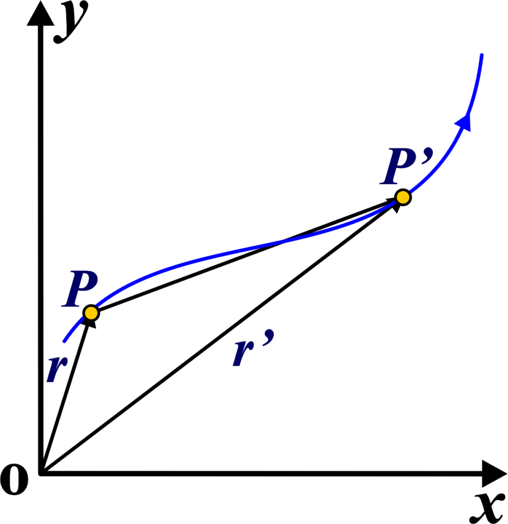
When something is moving around in a flat space (like on a piece of paper), we need a starting point to describe where it is. Let’s call this starting point O. Now, let’s say the object is at two different spots, P and P′, at different times, like t and t′. We can draw a straight line from O to P to show where the object is at time t. This line has an arrow at the end, which we call a position vector, and we’ll give it a symbol like “r”, so we say OP = r.
Then, for point P′, we draw another line from O to P′, and this is another position vector, which we call r′.
The length of the vector “r” tells us how far the object is from the starting point O, and the direction of the vector shows which way the object is from O.
Now, if the object moves from P to P′, we draw a new vector called PP′. This vector shows the straight line path from where the object started (P) to where it ended up (P′). We call this the displacement vector.
Equality of Vectors
Two vectors are equal if they have the same magnitude and direction, regardless of their initial points. When we say two vectors are equal, we mean they are identical in every way that matters for vectors. Here’s what that involves:
Same Magnitude: The magnitude is the ‘size’ or ‘length’ of the vector. If you think of a vector as an arrow, the magnitude is how long the arrow is. Two vectors are equal only if their magnitudes are the same.
Same Direction: Vectors have a direction, which is where the arrow is pointing. Two vectors are equal if they point in the same direction.
Independent of Initial Point: Here’s the cool part: vectors can start from different points and still be equal. It’s like two people in different cities looking at the same star. They’re in different places, but they’re looking in the same direction, at the same thing.
In math, we often write vectors with coordinates, like
\(\displaystyle\vec{A} = x\hat{i} + y\hat{j} + z\hat{k} \hspace{1cm} \) and
\(\displaystyle \vec{B} = p\hat{i} + q\hat{j} + r\hat{k} \hspace{1cm}\)
Vectors \(\displaystyle \vec{A} \) and \(\displaystyle \vec{B} \) are equal if (x = p), (y = q), and (z = r). This means each corresponding component must be the same. Equal vectors are denoted by the equality sign, just like numbers. So if \(\displaystyle\vec{A} \) and \(\displaystyle\vec{B} \) are equal, we write \(\displaystyle \vec{A} = \vec{B} \).
Example: Let’s say we have two vectors, \(\displaystyle\vec{A} \) and \(\displaystyle \vec{B} \). If \(\displaystyle\vec{A} \) is 5 units long and points north, and \(\displaystyle \vec{B} \) is also 5 units long and points north, then \(\displaystyle \vec{A} = \vec{B} \), even if \(\displaystyle \vec{A} \) starts in Paris and \(\displaystyle \vec{B} \) starts in Tokyo.
For vectors to be equal, they must have the same magnitude and direction, but they don’t need to have the same starting point.
Also Read: Kinematic Equations for Uniformly Accelerated Motion
Multiplication of Vector by Real Number
When we multiply a vector by a real number changes the magnitude of the vector but not its direction., we’re doing something called scalar multiplication. This is because a real number in this context is known as a scalar.
Imagine you have a vector, let’s call it \(\displaystyle\vec{v} \), and it represents something like velocity or force. Now, if we multiply this vector by a real number (scalar), say 3, we get \(\displaystyle3\vec{v} \). Here’s what happens:
- Magnitude: The magnitude (or length) of the vector gets multiplied by 3. If \(\displaystyle\vec{v} \) was 5 units long, \(\displaystyle 3\vec{v}\) will be 15 units long.
- Direction: The direction of the vector stays the same. If \(\displaystyle\vec{v} \) was pointing north, \(\displaystyle 3\vec{v}\) will also point north.
Think of it like stretching or shrinking a rubber band. The rubber band can get longer or shorter, but it still points in the same direction. That’s what scalar multiplication does to vectors.
Negative Scalars: What if we multiply by a negative number? If we have \(\displaystyle\vec{v} \) and we multiply it by -2, we get \(\displaystyle -2\vec{v} \). The vector’s magnitude is doubled, but its direction is reversed. It’s like turning the rubber band around to point the opposite way.
Zero Scalar: Multiplying any vector by zero gives us the zero vector, denoted as \(\displaystyle \vec{0} \). This vector has no magnitude and no direction—it’s just a point.
In terms of components, if \(\displaystyle\vec{v} = x\hat{i} + y\hat{j} \), then \(\displaystyle 3\vec{v} = 3x\hat{i} + 3y\hat{j} \). Each component of the vector is multiplied by the scalar.
Example: If a car is moving at a velocity of \(\displaystyle \vec{v} = 60 \text{ km/h} \) east, and we want to know the velocity if it triples its speed, we simply multiply by 3 to get \(\displaystyle 3\vec{v} = 180 \text{ km/h} \) east.
Multiplying a vector by a real number scales the vector’s magnitude without changing its direction. It’s a straightforward operation but a powerful tool in physics for understanding how quantities like forces and velocities can change in size while maintaining their direction.
Triangle Law of Vector Addition
If two vectors are represented as two sides of a triangle in sequence, the resultant vector is represented by the third side of the triangle taken in reverse order.
Imagine you’re on a treasure hunt. You walk 10 meters north, then 10 meters east. Instead of retracing your steps back to the start, you want to take the shortest path back to your starting point. This shortest path is like the resultant vector in the Triangle Law of Vector Addition.
Let’s say you have two vectors, \(\displaystyle\vec{A} \) and \(\displaystyle \vec{B} \). To add them using the Triangle Law:
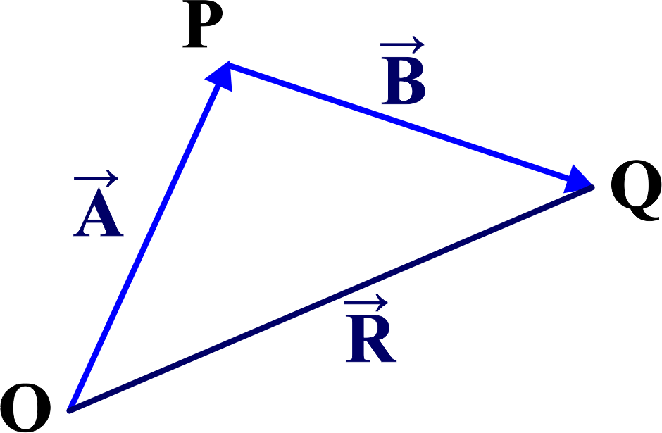
- Draw vector \(\displaystyle\vec{A} \) using an arrow.
- Now, draw vector \(\displaystyle\vec{B} \) starting from the head (the pointy end) of \(\displaystyle \vec{A} \).
- The resultant vector \(\displaystyle\vec{R} \) is drawn from the tail (the starting point) of \(\displaystyle\vec{A} \) to the head of \(\displaystyle\vec{B} \).
Mathematical Expression: Imagine two vectors, \(\displaystyle\vec{A} \) and \(\displaystyle \vec{B} \), that we want to add together. We’ll represent these vectors as arrows on a graph, with \(\displaystyle\vec{A} \) pointing in one direction \(\displaystyle\vec{B} \) pointing in another, and an angle ( \theta ) between them.
First, we draw vector \(\displaystyle\vec{A}\) as an arrow. Then, at the head of \(\displaystyle \vec{A} \), we draw vector \(\displaystyle\vec{B} \) such that the tail of \(\displaystyle \vec{B} \) meets the head of \(\displaystyle \vec{A} \).
We draw the resultant vector \(\displaystyle\vec{R} \) from the tail of \(\displaystyle \vec{A} \) to the head of \(\displaystyle\vec{B} \). This forms a triangle, and \(\displaystyle\vec{R} \) is the third side of the triangle, opposite the angle \(\displaystyle \theta \).
To find the magnitude of \(\displaystyle \vec{R} \), we use the Law of Cosines:
\(\displaystyle|\vec{R}|^2 = |\vec{A}|^2 + |\vec{B}|^2 – 2|\vec{A}||\vec{B}|\cos(180^\circ – \theta)\)
Since \(\displaystyle \cos(180^\circ – \theta) = -\cos(\theta) \), the equation becomes:
\(\displaystyle|\vec{R}|^2 = |\vec{A}|^2 + |\vec{B}|^2 + 2|\vec{A}||\vec{B}|\cos(\theta)\)
Taking the square root of both sides, we get the magnitude of the resultant vector:
\(\displaystyle |\vec{R}| = \sqrt{|\vec{A}|^2 + |\vec{B}|^2 + 2|\vec{A}||\vec{B}|\cos(\theta)}\)
This is the formula for the magnitude of the resultant vector when adding two vectors using the Triangle Law of Vector Addition.
To find the direction of \(\displaystyle \vec{R} \), we can use the Law of Sines or trigonometry to determine the angles within the triangle formed by \(\displaystyle \vec{A} \), \(\displaystyle \vec{B} \), and \(\displaystyle\vec{R} \).
This is how you derive the formula for the magnitude of the resultant vector when adding two vectors together. This law helps us find the total effect of two vectors when combined. For example, if one vector represents wind speed and direction, and the other represents a plane’s movement, the Triangle Law can give us the plane’s actual path over the ground.
Parallelogram Law of Vector Addition
If two vectors are represented by two adjacent sides of a parallelogram, the resultant vector is represented by the diagonal of the parallelogram starting from the same point.
The Parallelogram Law is a geometric approach to adding two vectors. It’s based on the idea that vectors are not just numbers; they have both magnitude and direction.
- Visualizing Vectors: Think of vectors as arrows. Each arrow has a length that represents the magnitude and a point that shows the direction.
- Creating a Parallelogram: When you have two vectors, you can place them tail-to-tail. Then, imagine drawing lines to form a parallelogram, using these vectors as adjacent sides.
- Finding the Resultant Vector: The diagonal of the parallelogram that starts from the common tail point of the two vectors gives us the resultant vector. This diagonal represents both the magnitude and direction of the sum of the two vectors.
Imagine two friends, Alice and Bob, are at a park. Alice walks 5 meters east, and Bob walks 8 meters north. Now, they want to meet up without retracing their steps. How do they find each other? They use the Parallelogram Law of Vector Addition!
The Parallelogram Law states that if two vectors are represented as adjacent sides of a parallelogram, the resultant vector is given by the diagonal of the parallelogram that starts from the common point of the two vectors.
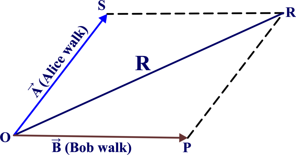
- Draw the Vectors: Start by drawing vector \(\displaystyle\vec{A} \) (Alice’s walk) and vector \(\displaystyle \vec{B} \) (Bob’s walk) with a common starting point.
- Form a Parallelogram: Next, extend these vectors to form a parallelogram. This means drawing lines parallel to \(\displaystyle \vec{A} \) and \(\displaystyle \vec{B} \) to complete the shape.
- Resultant Vector: The diagonal of the parallelogram that starts from the common point (where they started walking) represents the resultant vector \(\displaystyle \vec{R} \).
This law helps us find the combined effect of two different vectors. For example, if one vector represents the wind’s direction and speed, and the other represents a plane’s velocity, the Parallelogram Law can give us the plane’s actual path.
If \(\displaystyle\vec{A} \) and \(\displaystyle \vec{B} \) are our vectors, and \(\displaystyle \theta \) is the angle between them, the magnitude of the resultant vector \(\displaystyle \vec{R} \) can be found using the formula:
\(\displaystyle|\vec{R}| = \sqrt{|\vec{A}|^2 + |\vec{B}|^2 + 2|\vec{A}||\vec{B}|\cos\theta}\)
Example: Let’s say a boat is moving across a river. The engine gives it a velocity \(\displaystyle\vec{A} \) going straight across, and the river’s current gives it a velocity \(\displaystyle \vec{B} \) going downstream. The actual path of the boat will be the diagonal of the parallelogram formed by these two vectors.
The Parallelogram Law of Vector Addition is like finding the direct route to a destination when you’ve only been given the separate legs of the journey. It simplifies the route to a single vector that shows the overall effect of the two original vectors.
Addition and Subtraction of Vectors — Graphical Method
Vectors can be added or subtracted graphically by placing them head to tail and drawing the resultant vector from the start of the first vector to the end of the last vector.
Vector Addition: The Head-to-Tail Method
The “Head-to-Tail” method is a graphical way to add vectors, which are quantities that have both magnitude and direction. Here’s how it works:
- Draw the First Vector: Start by drawing the first vector (\(\displaystyle \vec{A} \)) on your paper or board. Make sure to draw an arrow that points in the correct direction and is proportional to the magnitude of the vector.
- Place the Second Vector: Now, take the second vector (\(\displaystyle \vec{B} \)) and draw it so that its tail starts at the head of the first vector. Again, the length and direction should be proportional to \(\displaystyle \vec{B} \)’s magnitude and direction.
- Draw the Resultant Vector: To find the sum of \(\displaystyle \vec{A} \) and \(\displaystyle \vec{B} \), you draw a new vector starting from the tail of \(\displaystyle \vec{A} \) (where you began) and ending at the head of \(\displaystyle \vec{B} \) (where you finished). This new vector is called the resultant vector (\(\displaystyle \vec{R} \)).
- Measure the Resultant Vector: Use a ruler to measure the length of \(\displaystyle \vec{R}\), which gives you the magnitude. Use a protractor to measure the angle of \(\displaystyle \vec{R} \) relative to a reference line, which gives you the direction.
Vector Subtraction: The Tail-to-Tail Method
When we talk about subtracting vectors, we’re essentially talking about finding a vector that, when added to the second vector, gives us the first vector. Here’s how we can visualize this using the Tail-to-Tail method:
- Identify the Vectors: First, we need to identify the vectors we want to subtract. Let’s say we have two vectors, \(\displaystyle \vec{A} ) and ( \vec{B} \), and we want to find \(\displaystyle \vec{A} – \vec{B} \).
- Draw the Vectors Tail-to-Tail: Instead of placing the vectors head-to-tail as we do for addition, we place them tail-to-tail. This means we draw both vectors so that their starting points (tails) are at the same point.
- Draw the Negative of the Second Vector: To subtract \(\displaystyle \vec{B} \) from \(\displaystyle \vec{A} \), we need to consider the negative of \(\displaystyle \vec{B} \), which we’ll call \(\displaystyle -\vec{B} \). This vector has the same magnitude as \(\displaystyle \vec{B} \) but points in the opposite direction.
- Complete the Triangle: Now, draw \(\displaystyle -\vec{B} \) starting from the tail of \(\displaystyle \vec{A} \). The head of \(\displaystyle -\vec{B} \) will point towards the head of \(\displaystyle \vec{A} \).
- Resultant Vector: The vector that starts at the head of \(\displaystyle -\vec{B} \) and ends at the head of \(\displaystyle \vec{A} \) is the resultant vector, which is the difference \(\displaystyle \vec{A} – \vec{B} \).
- Measure the Resultant Vector: Use a ruler to measure the length of the resultant vector to find its magnitude. Use a protractor to find the angle it makes with a reference line to determine its direction.
Remember, vectors are not just numbers; they have direction and magnitude, and the graphical method allows you to see the physical representation of these quantities. It’s a powerful tool for visual learners and an essential skill for any physics student.
Resolution of Vectors
Resolving vectors involves breaking down a vector into its horizontal and vertical components, usually using trigonometry.
Think of a vector as an arrow flying through space. It has a certain length (magnitude) and points in a specific direction. Now, imagine this arrow can be split into two smaller arrows, one pointing east and the other pointing north. These smaller arrows are what we call the components of the original vector.
In simple words, Vector resolution is the process of breaking down a vector into its components along specified axes, usually the horizontal (x-axis) and vertical (y-axis) axes. This is like finding out how much of the arrow’s flight is going eastward and how much is going northward.
Resolving a vector into components is super useful because it simplifies complex problems. For example, if you’re trying to figure out how a plane flying northeast is affected by wind blowing from the north, you can resolve the plane’s velocity into northward and eastward components to analyze the effects separately.
How to Resolve Vectors? Here’s a simple way to resolve a vector:
- Draw the Vector: Start by drawing your vector on graph paper, making sure it’s to scale.
- Choose Axes: Decide on your horizontal and vertical axes. These are usually aligned with the x and y directions on your graph paper.
- Draw Components: From the tip of your vector, draw a line straight down to the horizontal axis (x-axis) and another line straight across to the vertical axis (y-axis). These lines should create a right-angled triangle with your vector as the hypotenuse.
- Measure Components: The lengths of these lines are the magnitudes of your vector’s components. You can use trigonometry to calculate them if you know the angle your vector makes with the axes.
If your vector \(\displaystyle\vec{V} \) makes an angle (θ) with the horizontal axis, its components can be calculated as:
- Horizontal component (\(\displaystyle V_x): V_x = V \cos(\theta) \)
- Vertical component (\(\displaystyle V_y): V_y = V \sin(\theta) \)
where (V) is the magnitude of the original vector.
Example: Let’s say you have a force vector of 10 N making a 30° angle with the horizontal. Its horizontal component would be \(\displaystyle 10 \cos(30^\circ) \) and its vertical component would be \(\displaystyle 10 \sin(30^\circ) \).
Vector resolution helps us simplify and solve problems by breaking vectors into their horizontal and vertical parts. It’s like taking a journey and splitting it into the distance you travel east and the distance you travel north.
Unit Vector
A unit vector is a vector that has a magnitude (length) of exactly 1 unit and points in a particular direction. It’s like a compass arrow that’s always the same length, no matter where it points.
Unit vectors are super handy because they let us focus on the direction of a vector without worrying about its size. They’re like the pure essence of direction. Unit vectors are usually represented with a hat or cap symbol, like this: \(\displaystyle\hat{i} \), \(\displaystyle \hat{j} \), or \(\displaystyle\hat{k} \). These symbols represent unit vectors pointing along the x-axis, y-axis, and z-axis, respectively.
To turn any vector into a unit vector, you divide the vector by its magnitude. Here’s a simple formula:
\(\displaystyle\hat{v} = \frac{\vec{v}}{|\vec{v}|}\)
where \(\displaystyle \hat{v} \) is the unit vector, \(\displaystyle \vec{v} \) is the original vector, and \(\displaystyle |\vec{v}| \) is the magnitude of \(\displaystyle \vec{v} \).
Example: Let’s say we have a vector \(\displaystyle\vec{v} \) that’s 5 units long and points to the right. To make it a unit vector, we divide it by 5, and we get \(\displaystyle\hat{v} \), which is 1 unit long and still points to the right.
A unit vector tells us the direction of a vector and nothing else. It’s like saying “go straight ahead” without saying “how far” to go.
Vector Addition – Analytical Method
The analytical method of vector addition involves using algebra and geometry to add vectors together. This method is precise and allows us to calculate the resultant vector without drawing.
Steps for Analytical Vector Addition:
- Break Down Vectors into Components: First, we split each vector into its horizontal (x-axis) and vertical (y-axis) components. This is usually done using trigonometry, where the components of a vector \(\displaystyle\vec{A} \) are \(\displaystyle A_x = A \cos(\theta) \) and \(\displaystyle A_y = A \sin(\theta) \), with (θ) being the angle the vector makes with the horizontal axis.
- Add Components Separately: We then add the horizontal components of all vectors to get the total horizontal component (Rx) and do the same for the vertical components to get the total vertical component (Ry).
- Calculate the Resultant Vector: The resultant vector \(\displaystyle \vec{R} \) is found by combining the total horizontal and vertical components. Its magnitude can be calculated using the Pythagorean theorem:
\(\displaystyle |\vec{R}| = \sqrt{R_x^2 + R_y^2}\)
Its direction (angle (Φ) can be found using the arctangent function:
\(\displaystyle\phi = \arctan\left(\frac{R_y}{R_x}\right) \) - Express the Resultant Vector: Finally, the resultant vector \(\displaystyle\vec{R} \) can be expressed in component form as \(\displaystyle \vec{R} = R_x \hat{i} + R_y \hat{j} \), where \(\displaystyle\hat{i}\) and \(\displaystyle \hat{j} \) are the unit vectors in the direction of the x-axis and y-axis, respectively.
Example: Let’s say we have two vectors, \(\displaystyle\vec{A} \) and \(\displaystyle \vec{B} \). Vector \(\displaystyle \vec{A} \) has a magnitude of 5 units at an angle of 30° from the x-axis, and vector \(\displaystyle \vec{B} \) has a magnitude of 5 units at an angle of 120° from the x-axis.
For ( \vec{A} ):
- \(\displaystyle A_x = 5 \cos(30°) \)
- \(\displaystyle A_y = 5 \sin(30°) \)
For \(\displaystyle \vec{B} \):
- \(\displaystyle B_x = 5 \cos(120°) \)
- \(\displaystyle B_y = 5 \sin(120°) \)
Add the components:
- \(\displaystyle R_{x} = A_{x} + B_{x} \)
- \(\displaystyle R_{y} = A_{y} + B_{y} \)
Then find the magnitude and direction of \(\displaystyle \vec{R} \) using the formulas above. This analytical method is powerful because it allows us to add vectors numerically and is especially useful when dealing with more than two vectors or when precise calculations are required.
Solved Examples
Problem 1: A person walks 4 km east and then 3 km north. Determine the magnitude and direction of the resultant displacement vector.
Solution: Let’s denote:
- The eastward displacement vector as (\(\displaystyle\vec{A} = 4 \hat{i}\) ) km
- The northward displacement vector as (\(\displaystyle\vec{B} = 3 \hat{j} \)) km
The resultant displacement vector ( \vec{R} ) is given by:
\(\displaystyle \vec{R} = \vec{A} + \vec{B} = 4 \hat{i} + 3 \hat{j} \, \text{km} \)
Magnitude of (\(\displaystyle\vec{R}\)):
\(\displaystyle |\vec{R}| = \sqrt{(4)^2 + (3)^2} = \sqrt{16 + 9} = \sqrt{25} = 5 \, \text{km} \)
Direction of (\(\displaystyle\vec{R}\)):
\(\displaystyle \theta = \tan^{-1} \left( \frac{3}{4} \right) \)
\(\displaystyle \theta = \tan^{-1} \left( 0.75 \right) \approx 36.87^\circ \)
The magnitude of the resultant displacement vector is 5 km, and the direction is (36.87∘) north of east.
Problem 2: Two vectors (\(\displaystyle\vec{A}\)) and (\(\displaystyle\vec{B}\)) have magnitudes of 5 units and 5 units, respectively. If (\(\displaystyle\vec{A} = 5 \hat{i} + 2 \hat{j}\)) and (\(\displaystyle\vec{B} = 5 \hat{i} + 2 \hat{j}\)), are the vectors equal?
Solution: Vectors (\(\displaystyle\vec{A}\)) and (\(\displaystyle\vec{B}\)) are equal if they have the same magnitude and direction. Given:
\(\displaystyle \vec{A} = 5 \hat{i} + 2 \hat{j} \)
\(\displaystyle \vec{B} = 5 \hat{i} + 2 \hat{j} \)
Since the components of (\(\displaystyle\vec{A}\)) and (\(\displaystyle\vec{B}\)) are identical, we can conclude:
\(\displaystyle \vec{A} = \vec{B} \)
Yes, the vectors (\(\displaystyle\vec{A}\)) and (\(\displaystyle\vec{B}\)) are equal.
Problem 3: Two vectors (\(\displaystyle\vec{A}\)) and (\(\displaystyle\vec{B}\)) have magnitudes of 7 units and 24 units, respectively. If they are at right angles to each other, find the magnitude of the resultant vector.
Solution: Using the triangle law of vector addition for vectors at right angles:
\(\displaystyle |\vec{R}| = \sqrt{|\vec{A}|^2 + |\vec{B}|^2} \)
\(\displaystyle |\vec{R}| = \sqrt{7^2 + 24^2} = \sqrt{49 + 576} = \sqrt{625} = 25 \, \text{units} \)
The magnitude of the resultant vector is 25 units.
Problem 4: Two vectors (\(\displaystyle\vec{A}\)) and (\(\displaystyle\vec{B}\)) have magnitudes of 8 units and 6 units, respectively, and the angle between them is (60∘). Find the magnitude of the resultant vector using the parallelogram law of vector addition.
Solution: Using the parallelogram law of vector addition:
\(\displaystyle |\vec{R}| = \sqrt{|\vec{A}|^2 + |\vec{B}|^2 + 2|\vec{A}||\vec{B}| \cos \theta} \)
\(\displaystyle |\vec{R}| = \sqrt{8^2 + 6^2 + 2 \cdot 8 \cdot 6 \cdot \cos 60^\circ} \)
\(\displaystyle |\vec{R}| = \sqrt{64 + 36 + 48 \cdot 0.5} \)
\(\displaystyle |\vec{R}| = \sqrt{64 + 36 + 24}\)
\(\displaystyle |\vec{R}| = \sqrt{124} \)
\(\displaystyle |\vec{R}| \approx 11.14 \, \text{units} \)
The magnitude of the resultant vector is approximately 11.14 units.
Problem 5: Resolve the vector (\(\displaystyle\vec{A} = 10 \, \text{units} \)) making an angle of (30∘) with the x-axis into its horizontal and vertical components.
Solution: The horizontal component (Ax) and vertical component (Ay) are given by:
\(\displaystyle A_x = A \cos \theta \)
\(\displaystyle A_y = A \sin \theta \)
Given: \(\displaystyle A = 10 \, \text{units}, \, \theta = 30^\circ \); \(\displaystyle A_x = 10 \cos 30^\circ = 10 \times \frac{\sqrt{3}}{2} = 5\sqrt{3} \, \text{units} \approx 8.66 \, \text{units} \); \(\displaystyle A_y = 10 \sin 30^\circ = 10 \times \frac{1}{2} = 5 \, \text{units} \)
The horizontal component is (8.66 units) and the vertical component is (5 units).
Problem 6: Find the unit vector in the direction of the vector (\(\displaystyle\vec{A} = 3 \hat{i} + 4 \hat{j} \)).
Solution: The magnitude of vector (\(\displaystyle\vec{A}\)) is:
\(\displaystyle |\vec{A}| = \sqrt{3^2 + 4^2} = \sqrt{9 + 16} = \sqrt{25} = 5 \)
The unit vector (\(\displaystyle\hat{A}\)) is given by:
\(\displaystyle \hat{A} = \frac{\vec{A}}{|\vec{A}|} \)
\(\displaystyle \hat{A} = \frac{3 \hat{i} + 4 \hat{j}}{5} \)
\(\displaystyle \hat{A} = \frac{3}{5} \hat{i} + \frac{4}{5} \hat{j} \)
The unit vector in the direction of (\(\displaystyle\vec{A}\)) is (\(\displaystyle\frac{3}{5} \hat{i} + \frac{4}{5} \hat{j}\)).
FAQs
What are scalars and vectors, and how do they differ?
Scalars are quantities that have magnitude only, such as mass, temperature, and speed. Vectors, on the other hand, are quantities that have both magnitude and direction, such as displacement, velocity, and force. Scalars can be represented by single numbers, while vectors require both magnitude and direction for a complete description.
Can you provide examples of scalar and vector quantities in everyday life?
Examples of scalar quantities include distance traveled, time taken, and temperature. Examples of vector quantities include displacement (distance with direction), velocity (speed with direction), and force (strength with direction).
How do unit vectors help in understanding vectors?
Unit vectors have a magnitude of one and point in a specific direction. They are used to indicate direction and can help in breaking down vectors into their components, making calculations easier and more intuitive.
How do we represent vectors graphically?
Vectors are often represented graphically using arrows. The length of the arrow represents the magnitude of the vector, while the direction of the arrow indicates the direction of the vector. The starting point of the arrow is typically the tail, and the ending point is the head.
What are the rules for adding and subtracting vectors?
Vectors can be added or subtracted using the parallelogram law or the triangle law. In the parallelogram law, vectors are added by constructing a parallelogram where the two vectors are adjacent sides, and the diagonal of the parallelogram represents the resultant vector. In the triangle law, vectors are added by placing them head-to-tail, and the resultant vector is the vector connecting the initial point of the first vector to the final point of the last vector.
Can scalar quantities be negative?
Yes, scalar quantities can be negative if they represent a measurement that has a direction associated with it. For example, if we define displacement to the left as negative and displacement to the right as positive, a displacement of -5 meters indicates movement to the left.
How do we distinguish between scalar and vector quantities in equations?
In equations, scalar quantities are represented by regular symbols or variables without any arrows or bold fonts. For example, “t” represents time, “m” represents mass. Vector quantities, on the other hand, are typically represented by bold symbols or symbols with arrows above them. For example, “v” with an arrow represents velocity, and “F” with an arrow represents force.
Are there any physical quantities that can be either scalar or vector depending on context?
Yes, some physical quantities can be either scalar or vector depending on the context. For example, speed is a scalar quantity because it only has magnitude, while velocity is a vector quantity because it has both magnitude and direction. Similarly, distance is a scalar quantity, but displacement is a vector quantity.