1. The Core of Measurement
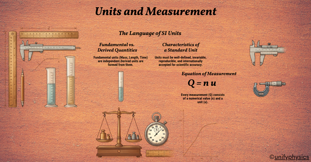
Every physical quantity (Q) is measured as a product of its numerical value (n) and its standard unit (u).
- The Golden Rule: The magnitude of a physical quantity remains constant regardless of the system of units used.
- Formula: n₁u₁ = n₂u₂
- (Explanation: If you switch to a smaller unit, the numerical value becomes larger, e.g., 1 kg = 1000 g).
2. Base Quantities & Their Dimensions
To understand how derived quantities are built from fundamental ones, we use dimensions.
- Definition: Dimensions are the powers to which the fundamental units (like Mass, Length, and Time, written as M, L, and T) are raised to represent a physical quantity.
- Key Insight: Dimensions indicate the nature of the physical quantity, not its magnitude or numerical value.
- Example Explanation: Area is calculated as Length × Breadth. Since both are lengths, the dimensions of Area are [L¹] × [L¹] = [L²]. To write it completely in terms of mass, length, and time, it is expressed as [M⁰ L² T⁰].
Dimensional Formula & Equation
- Dimensional Formula: It is an expression showing the powers of mass, length, and time that indicates exactly how a physical quantity depends on the fundamental quantities.
- Example: For Speed (Distance / Time), the dimensional formula is [M⁰ L¹ T⁻¹]. This tells us that speed depends on length (L) and time (T), but is completely independent of mass (M).
- Dimensional Equation: When you equate a physical quantity to its dimensional formula, you get a dimensional equation.
- Example: Density = [M¹ L⁻³ T⁰].
Classification of Physical Quantities
Based on dimensional analysis, physical quantities are grouped into four distinct categories.
- Dimensional Constants: Quantities that have a fixed value and possess dimensions.
- Examples: Planck’s constant, Gas constant, Universal gravitational constant.
- Dimensional Variables: Quantities that possess dimensions but do not have a fixed value.
- Examples: Velocity, Acceleration, Force.
- Dimensionless Constants: Quantities that have a fixed value but do not possess any dimensions.
- Examples: Numbers (1, 2, 3…), π, e.
- Dimensionless Variables: Quantities that have variable values but do not possess dimensions.
- Examples: Angle, Strain, Specific gravity.
To master dimensional analysis, you must memorize the fundamental quantities and their specific dimensional symbols.
| Fundamental Quantity | SI Unit | Dimensional Symbol |
| Mass | Kilogram (kg) | [M¹ L⁰ T⁰] or [M] |
| Length | Metre (m) | [M⁰ L¹ T⁰] or [L] |
| Time | Second (s) | [M⁰ L⁰ T¹] or [T] |
| Temperature | Kelvin (K) | [K] |
| Electric Current | Ampere (A) | [A] |
| Luminous Intensity | Candela (cd) | [cd] |
| Amount of Substance | Mole (mol) | [mol] |
Note: Supplementary units like Plane Angle (Radian) and Solid Angle (Steradian) are dimensionless ratios.
3. High-Yield Dimensional Formulas
Derived quantities are built from base quantities. Here is a quick-reference table of the most frequently tested physical quantities:
| Physical Quantity | Formula / Relation | Dimensional Formula | SI Unit |
| Velocity / Speed | Distance / Time | [M⁰ L¹ T⁻¹] | m/s |
| Acceleration | Velocity / Time | [M⁰ L¹ T⁻²] | m/s² |
| Force | Mass × Accel. | [M¹ L¹ T⁻²] | Newton (N) |
| Work / Energy | Force × Distance | [M¹ L² T⁻²] | Joule (J) |
| Power | Work / Time | [M¹ L² T⁻³] | Watt (W) |
| Pressure / Stress | Force / Area | [M¹ L⁻¹ T⁻²] | Pascal (Pa) or N/m² |
| Momentum / Impulse | Mass × Velocity | [M¹ L¹ T⁻¹] | kg m/s |
| Surface Tension | Force / Length | [M¹ L⁰ T⁻²] | N/m |
| Coefficient of Viscosity | Force × Dist / (Area × Vel) | [M¹ L⁻¹ T⁻¹] | N s/m² |
| Strain | Change in dim. / Orig. dim. | [M⁰ L⁰ T⁰] | No Unit |
4. Dimensional Analysis & Its Rules
A. Principle of Homogeneity:
- Concept: You can only add or subtract physical quantities that have the exact same dimensions.
- Application: In any equation (e.g., A + B = C – D), the dimensions of A, B, C, and D must be identical.
B. Conversion of System of Units:
- Formula: n₂ = n₁ [M₁/M₂]ᵃ [L₁/L₂]ᵇ [T₁/T₂]ᶜ
- (Explanation: Used to convert a quantity with dimensional formula [Mᵃ Lᵇ Tᶜ] from System 1 to System 2).
Dimensions & SI Units of Physical Quantities
Here is a high-yield table combining the physical quantity, its basic formula, dimensions, and SI unit.
| Physical Quantity | Basic Formula | Dimensions | SI Unit |
| Area | Length × Breadth | [M⁰ L² T⁰] | Metre² |
| Volume | Length × Breadth × Height | [M⁰ L³ T⁰] | Metre³ |
| Density | Mass / Volume | [M¹ L⁻³ T⁰] | Kg/m³ |
| Speed / Velocity | Distance / Time | [M⁰ L¹ T⁻¹] | m/s |
| Acceleration | Velocity / Time | [M⁰ L¹ T⁻²] | m/s² |
| Momentum | Mass × Velocity | [M¹ L¹ T⁻¹] | Kg ms⁻¹ |
| Force | Mass × Acceleration | [M¹ L¹ T⁻²] | Newton (N) |
| Work | Force × Distance | [M¹ L² T⁻²] | Joule (J) |
| Power | Work / Time | [M¹ L² T⁻³] | Watt (W) |
| Energy (all forms) | Stored work | [M¹ L² T⁻²] | Joule (J) |
| Pressure / Stress | Force / Area | [M¹ L⁻¹ T⁻²] | N/m² or Nm⁻² |
| Impulse | Force × Time | [M¹ L¹ T⁻¹] | Ns |
| Moment of Force | Force × Distance | [M¹ L² T⁻²] | Nm |
| Strain | Change in dim. / Original dim. | [M⁰ L⁰ T⁰] | No unit |
| Modulus of Elasticity | Stress / Strain | [M¹ L⁻¹ T⁻²] | Nm⁻² |
| Surface Tension | Force / Length | [M¹ L⁰ T⁻²] | N/m |
| Surface Energy | Energy / Area | [M¹ L⁰ T⁻²] | Joule/m² |
| Coefficient of Viscosity | Force × Dist. / (Area × Vel.) | [M¹ L⁻¹ T⁻¹] | N/m² * |
| Moment of Inertia | Mass × (Radius of gyration)² | [M¹ L² T⁰] | Kg-m² |
| Angular Velocity | Angle / Time | [M⁰ L⁰ T⁻¹] | Rad per sec |
| Frequency | 1 / Time period | [M⁰ L⁰ T⁻¹] | Hertz |
5. Error Analysis
Every measurement has uncertainty. Here is how you calculate it:
A. Types of Errors:
- Absolute Error: Δa = atrue – ameasured
- Mean Absolute Error (Δamean): The arithmetic mean of the magnitudes of all absolute errors.
- Relative / Fractional Error: Δamean / amean (Ratio of mean absolute error to the true average value).
- Percentage Error: (Δamean / amean) × 100%
B. Combination of Errors:
- Addition / Subtraction: Maximum absolute errors are always added.
- If X = A ± B, then ΔX = ΔA + ΔB
- Multiplication / Division: Maximum relative (fractional) errors are always added.
- If X = A × B or X = A / B, then ΔX/X = ΔA/A + ΔB/B
- Quantities Raised to a Power: The power is multiplied by the fractional error.
- If X = (Ap × Bq) / Cr, then ΔX/X = p(ΔA/A) + q(ΔB/B) + r(ΔC/C)
6. Measuring Instruments
A. Vernier Callipers (For precise linear lengths):
- Least Count (LC): 1 MSD – 1 VSD(MSD = Main Scale Division, VSD = Vernier Scale Division).
- Total Reading: MSR + (VSR × LC)(MSR = Main Scale Reading, VSR = Vernier scale division coinciding exactly with a main scale line).
B. Screw Gauge (For spherical/cylindrical objects like wires):
- Least Count (LC): Pitch / Total divisions on circular scale(Pitch is the linear distance the screw moves in one full rotation).
- Total Reading: LSR + (CSR × LC)(LSR = Linear scale reading, CSR = Circular scale reading coinciding with the reference line).
C. Zero Error Correction (Applies to both):
- Rule: Correct Reading = Measured Reading – Zero Error(Explanation: Always subtract the zero error, retaining its positive or negative sign).
Also Read: Heat, Internal Energy, and Work
Solved Problem
Question 1: In the van der Waals gas equation (P + a/V²)(V – b) = RT, where P is pressure, V is volume, R is the universal gas constant, and T is temperature. Find the dimensional formulas of the constants a and b.
Solution: According to the Principle of Homogeneity, only physical quantities with the same dimensions can be added or subtracted from one another.
First (Find b): In the term (V – b), the constant b is subtracted from Volume (V). Therefore, the dimensions of b must be identical to the dimensions of Volume.
Dimension of Volume (V) = [M⁰ L³ T⁰]
Dimension of b = [M⁰ L³ T⁰]
Now (Find a): In the term (P + a/V²), the quantity a/V² is added to Pressure (P). Therefore, a/V² must have the same dimensions as Pressure.
Dimension of Pressure (P) = Force / Area = [M¹ L⁻¹ T⁻²].
Dimension of Volume squared (V²) = [L³]² = [L⁶]
Since [a] / [V²] = [P], we get [a] = [P] × [V²]
[a] = [M¹ L⁻¹ T⁻²] × [L⁶]
Dimension of a = [M¹ L⁵ T⁻²]
Question 2: The velocity (v) of a particle at time (t) is given by the equation v = at + b/(t + c). Find the dimensional formulas for the constants a, b, and c.
Solution: By the principle of homogeneity, every individual term in an equation must have the exact same dimensions.
Step 1 (Find c): In the denominator (t + c), c is added to time (t). Thus, c must have the dimension of time.
Dimension of c = [M⁰ L⁰ T¹]
Step 2 (Find a): The term at must have the same dimensions as velocity (v).
[a] × [t] = [v]
[a] × [T¹] = [M⁰ L¹ T⁻¹]
[a] = [M⁰ L¹ T⁻¹] / [T¹]
Dimension of a = [M⁰ L¹ T⁻²] (This is the dimension of acceleration).
Step 3 (Find b): The entire term b/(t + c) must also have the dimensions of velocity (v).
[b] / [T¹] = [M⁰ L¹ T⁻¹]
[b] = [M⁰ L¹ T⁻¹] × [T¹]
Dimension of b = [M⁰ L¹ T⁰] (This is the dimension of length).
Question 3: Using dimensional analysis, convert a force of 1 Newton into its CGS unit (dyne).
Solution: The dimensional formula for Force is [M¹ L¹ T⁻²]. Here, the powers are: a = 1, b = 1, c = -2. We use the conversion formula: n₂ = n₁ [M₁/M₂]ᵃ [L₁/L₂]ᵇ [T₁/T₂]ᶜ
System 1 (SI Unit – Newton): n₁ = 1, M₁ = 1 kg, L₁ = 1 m, T₁ = 1 s.
System 2 (CGS Unit – Dyne): n₂ = ?, M₂ = 1 g, L₂ = 1 cm, T₂ = 1 s.
Calculation:
n₂ = 1 × [1 kg / 1 g]¹ × [1 m / 1 cm]¹ × [1 s / 1 s]⁻²
n₂ = 1 × [1000 g / 1 g]¹ × [100 cm / 1 cm]¹ × [1]
n₂ = 1000 × 100 = 100,000 = 10⁵.
Answer: 1 Newton = 10⁵ dynes.
Question 4: A physical quantity X is calculated using the relation: X = (a² × b³) / (c × √d).
If the percentage errors in the measurement of a, b, c, and d are 1%, 2%, 3%, and 4% respectively, calculate the maximum percentage error in X.
Solution:
The relation can be rewritten with powers as: X = (a² × b³) / (c¹ × d0.5).
Using the shortcut rule for errors raised to a power (powers are multiplied by the fractional error and maximum errors are always added):
Formula: ΔX/X × 100 = 2(Δa/a × 100) + 3(Δb/b × 100) + 1(Δc/c × 100) + 0.5(Δd/d × 100)
Substitute the given percentage errors:
Percentage error in X = 2(1%) + 3(2%) + 1(3%) + 0.5(4%)
Percentage error in X = 2% + 6% + 3% + 2%
Answer: The maximum percentage error in X is 13%.
Question 5: In a Vernier Calliper, 10 divisions of the Vernier scale (VSD) perfectly coincide with 9 divisions of the main scale (MSD). If 1 main scale division is exactly 1 mm, calculate the Least Count (LC) of the instrument.
Solution:
Step 1: Identify the value of 1 Main Scale Division (MSD).
1 MSD = 1 mm.
Step 2: Find the value of 1 Vernier Scale Division (VSD) in terms of MSD.
10 VSD = 9 MSD
1 VSD = 9/10 MSD = 0.9 MSD
Step 3: Use the Least Count formula: LC = 1 MSD – 1 VSD.
LC = 1 MSD – 0.9 MSD
LC = 0.1 MSD
Step 4: Convert to the final unit.
LC = 0.1 × 1 mm = 0.1 mm.
Answer: The Least Count is 0.1 mm (or 0.01 cm).